Visualization Guide

What NOT to do

Unfortunately, the first thing that ParaView shows when you open a particle field is a "scatter plot" full of confusing colors like this:

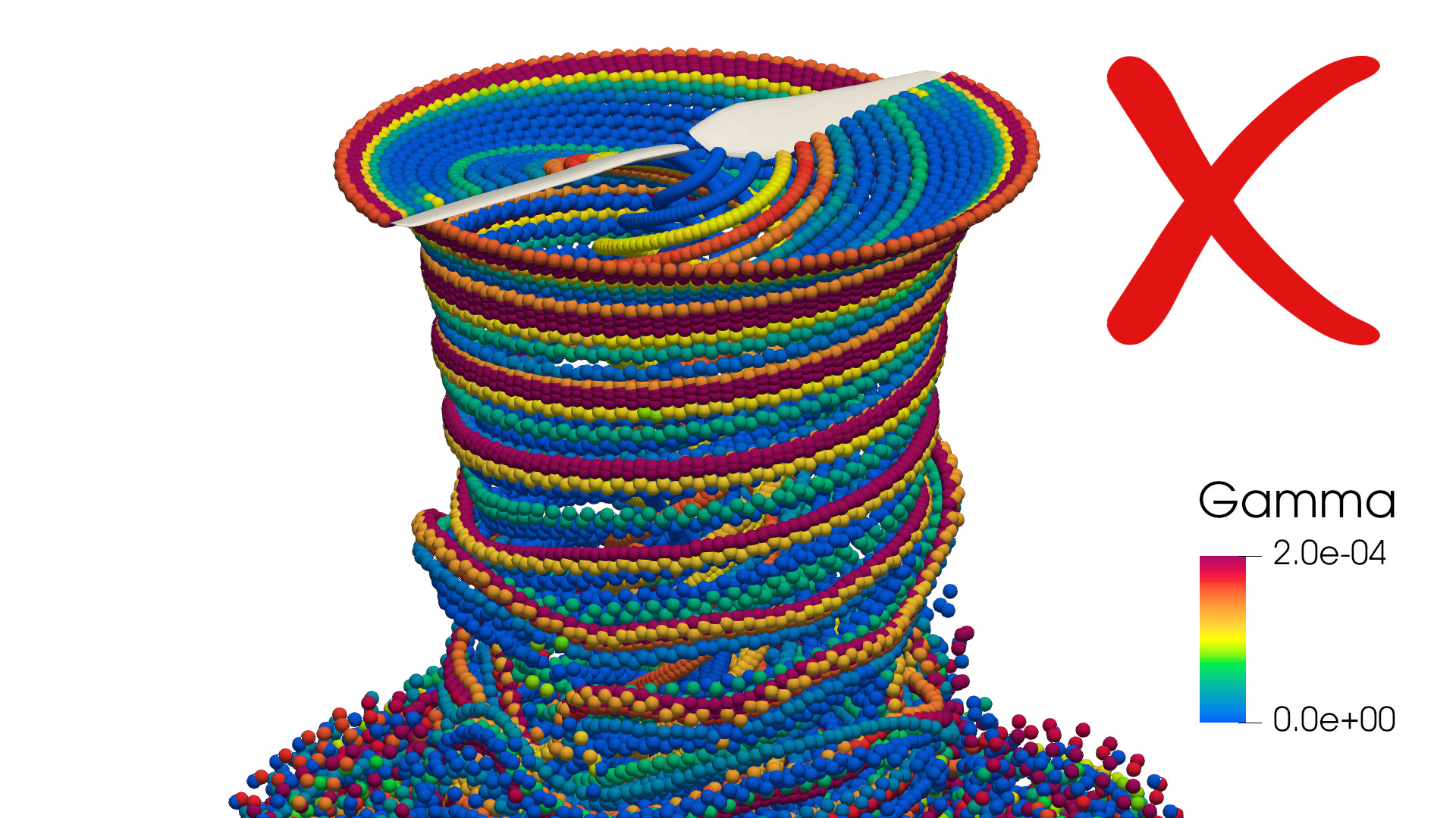
Not surprisingly, the VPM literature is full of these visualizations, which provide very little information about the simulation. Poor colormap aside, why is this a bad visualization? Even though we are coloring the strengths of the particles, one must remember that the particle strength $\boldsymbol\Gamma$ is the integral of the vorticity over the volume that is discretized by the particle, $\boldsymbol\Gamma = \int\limits_{\mathrm{Vol}} \boldsymbol\omega \mathrm{d}V$. This is equivalent to the average vorticity times the volume, $\boldsymbol\Gamma = \overline{\boldsymbol\omega} \mathrm{Vol}$, which means that the particle strength is proportional to the volume that it discretizes. Thus, the particle strength has no physical significance, but is purely a numerical artifact. (In fact, $\boldsymbol\Gamma$ are nothing more than the coefficients of the radial basis function that reconstructs the vorticity field as $\overline{\boldsymbol\omega}\left( \mathbf{x}\right) \approx \sum\limits_p \boldsymbol{\Gamma}_p \zeta_{\sigma_p}(\mathbf{x}-\mathbf{x}_p)$.)

Another VPM visualization that is commonly found in the literature simply shows the position of the particles:

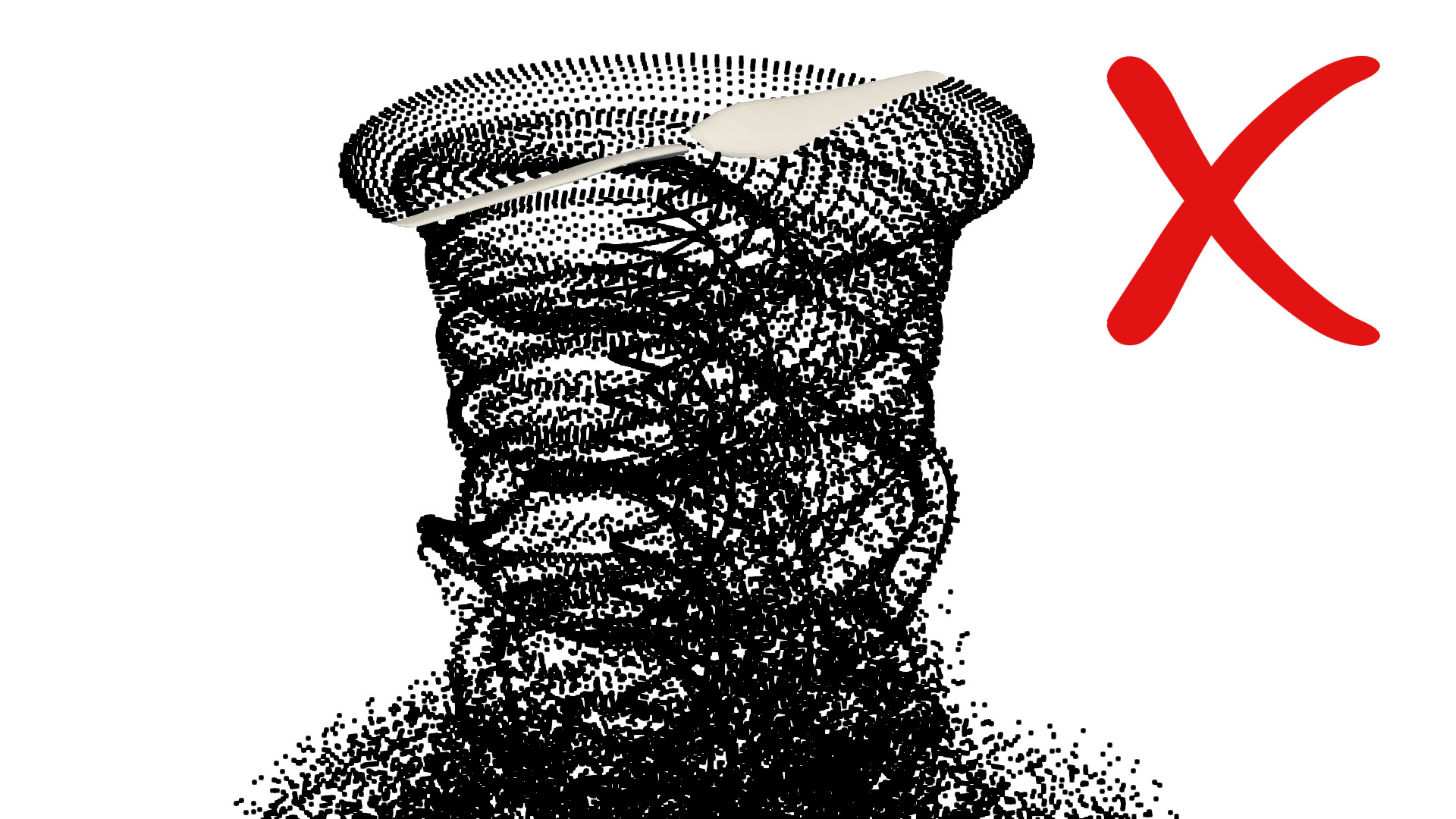
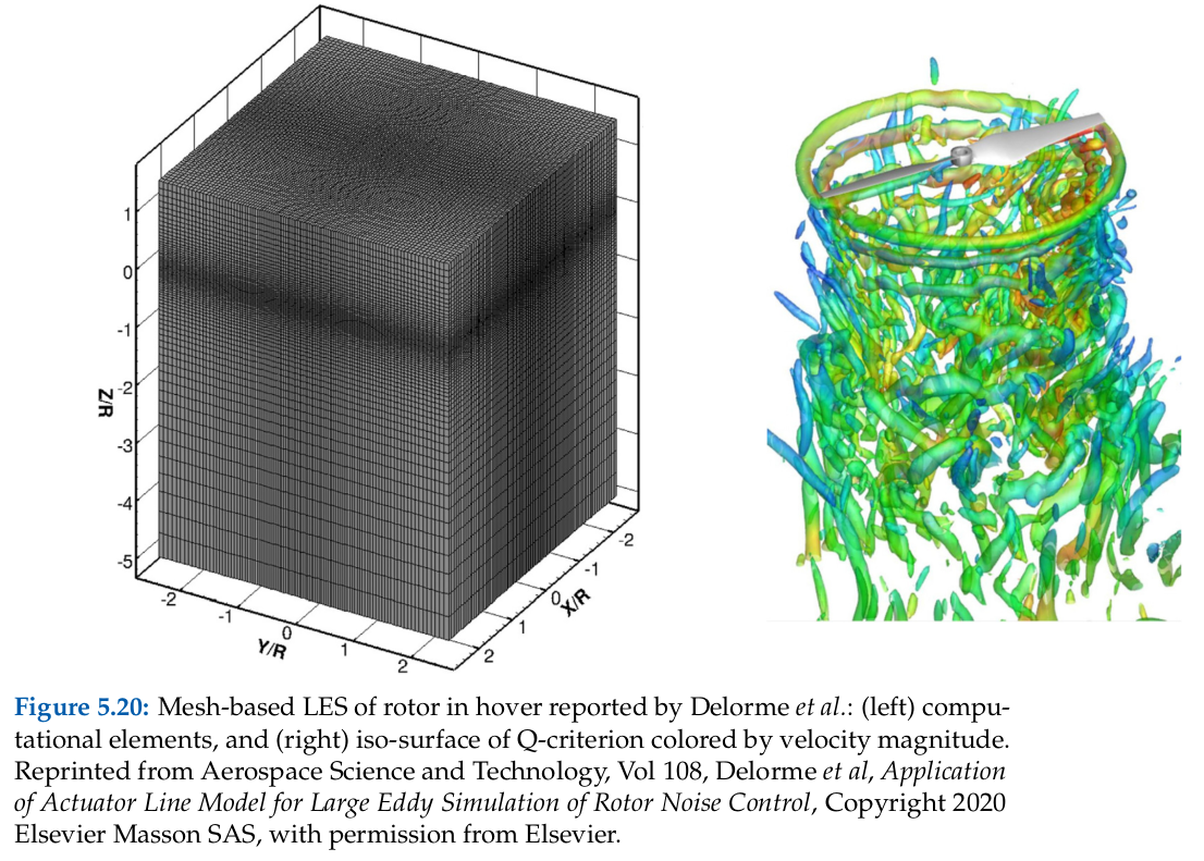
Why is this a bad visualization? Even though its intent is to depict the flow field by taking advantage of the fact that particles follow streamlines and vortical structures, what is actually visualized is the spatial discretization. After all, we are just looking at the position of the computational elements. Here is an equivalent visualization of the computational elements in a mesh-based simulation of the same rotor in hover:

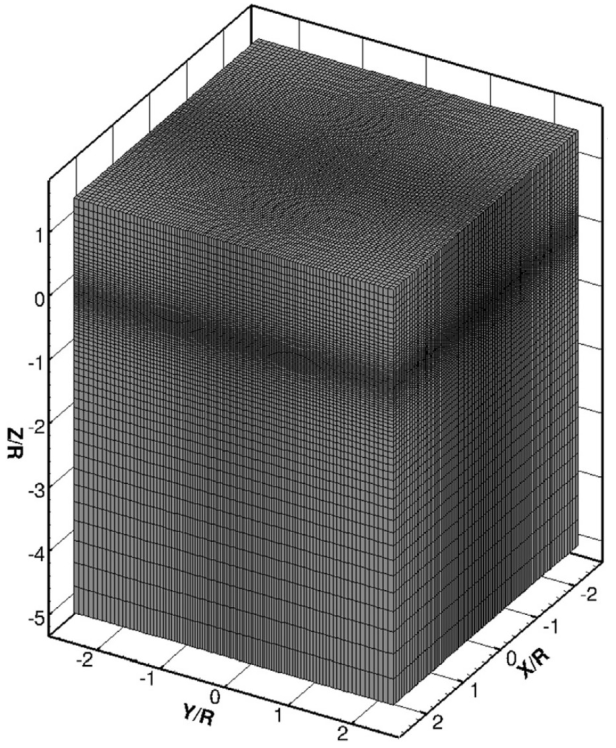
Not very insightful, is it?

What we recommend

In order to correctly visualize the flow field that is predicted by the VPM solver, one must reconstruct the vorticity field using the particles as a radial basis function and compute the velocity field using the Biot-Savart law. This can be computationally intensive and is not a streamlined process.

Alternatively, a quick visualization that sheds insights into both the flow field and the discretization is to make glyphs that point in the direction of $\boldsymbol\Gamma$ (arrows scaled by magnitude), thus forming the vortex lines:

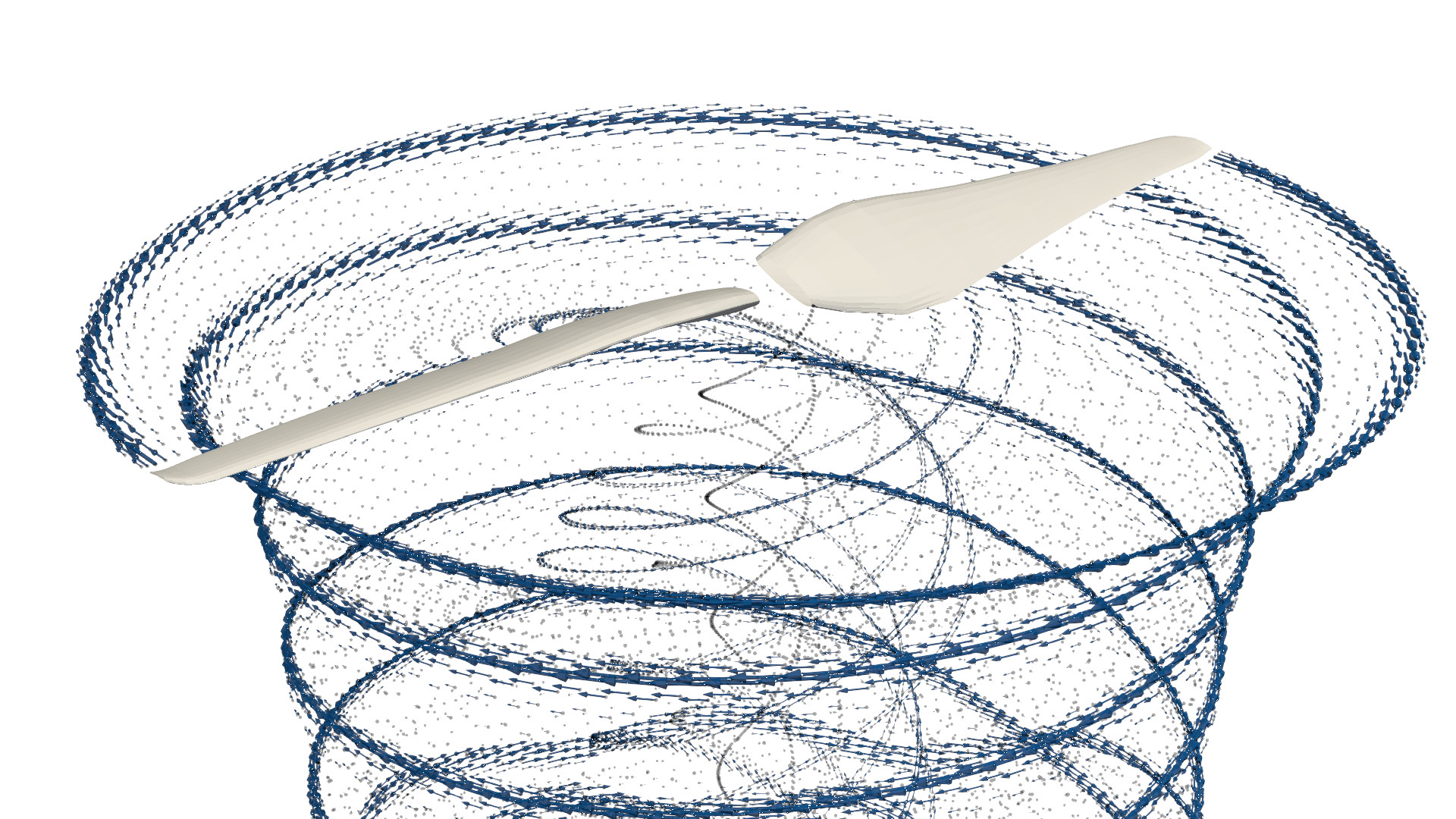
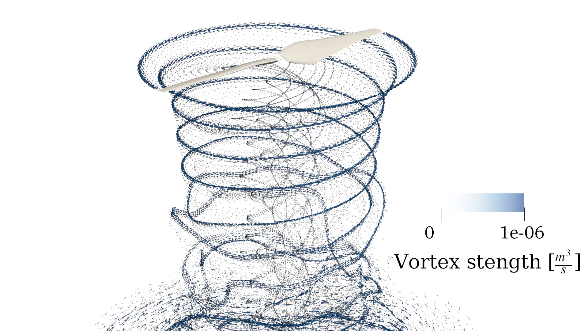
This type of visualization has four advantages:

• It clearly reveals the vortical structure (vortex lines) in a quick glimpse
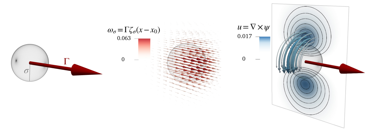
• One can envision the velocity field around the vortex lines using the right hand rule (Biot-Savart law shown below)
• Adding small points at the position of each particle gives us an idea of the spatial resolution around vortices
• One can easily spot if the simulation is becoming numerically unstable since blown-up particles become giant arrows

Fluid domain

While the "glyph" visualization shown above uses the native variables that are computed and outputted by the VPM ($\boldsymbol\Gamma_p$ and $\mathbf{x}_p$), the full fluid domain can be computed from the particle field in postprocessing. This is done using the particles as a radial basis function to construct a continuous and analytical vorticity field $\boldsymbol\omega(\mathbf{x})$, and the Biot-Savart law is used to obtain a continuous and analytical velocity field $\mathbf{u}(\mathbf{x})$. Since $\boldsymbol\omega(\mathbf{x})$ and $\mathbf{u}(\mathbf{x})$ are analytical functions, their values and their derivatives can be calculated anywhere in space.

FLOWUnsteady provides the function uns.computefluiddomain that reads a simulation and processes it to generate its fluid domain. See the Rotor in Hover tutorial for an example on how to use uns.computefluiddomain.

Whenever reporting results, we recommend showing the vortex elements (glyph visualization) and the fluid domain side by side to give a clear idea of the spatial resolution and the resulting flow field (see example below), which is custom in conventional mesh-based CFD.

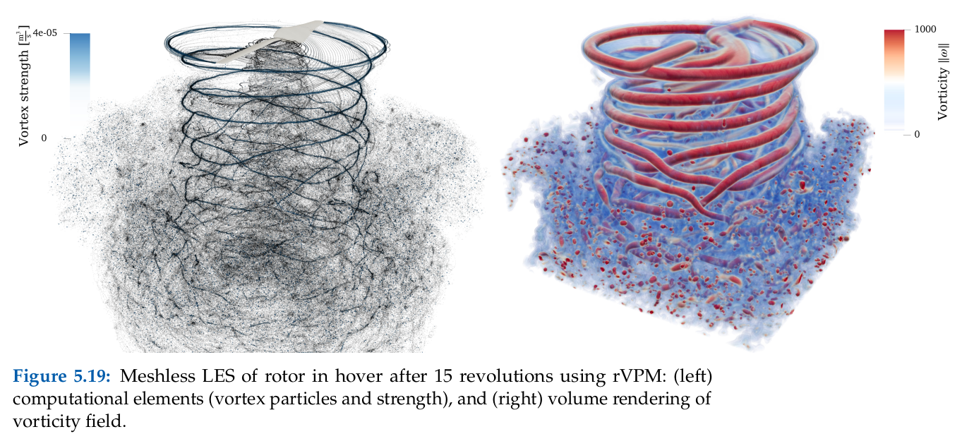
Here is an example of a simulation superimposing the particle field and the resulting fluid domain: