Simple Wing
In this example we simulate a $45^\circ$ swept-back wing at an angle of attack of $4.2^\circ$. In the process we exemplify the basic structure of simulations, which is always the same, no matter how complex the simulation might be. The structure consists of six steps:
(1) Vehicle Definition: Generate the geometry of the vehicle and declare each vehicle subsystem in a
FLOWUnsteady.VLMVehicleobject
(2) Maneuver Definition: Generate functions that prescribe the kinematics of the vehicle and specify the control inputs for tilting and rotor subsystems in a
FLOWUnsteady.KinematicManeuverobject
(3) Simulation Definition: A
FLOWUnsteady.Simulationobject is generated stating the vehicle, maneuver, and total time and speed at which to perform the maneuver
(4) Monitors Definitions: Functions are generated for calculating, monitoring, and outputting different metrics throughout the simulation
(6) Viz and Postprocessing: The simulation is visualized in Paraview and results are postprocessed
While in this example we show the basic structure without much explanation, in subsequent examples we will dive into the details and options of each step (which are also listed in the API Guide).
#=##############################################################################
# DESCRIPTION
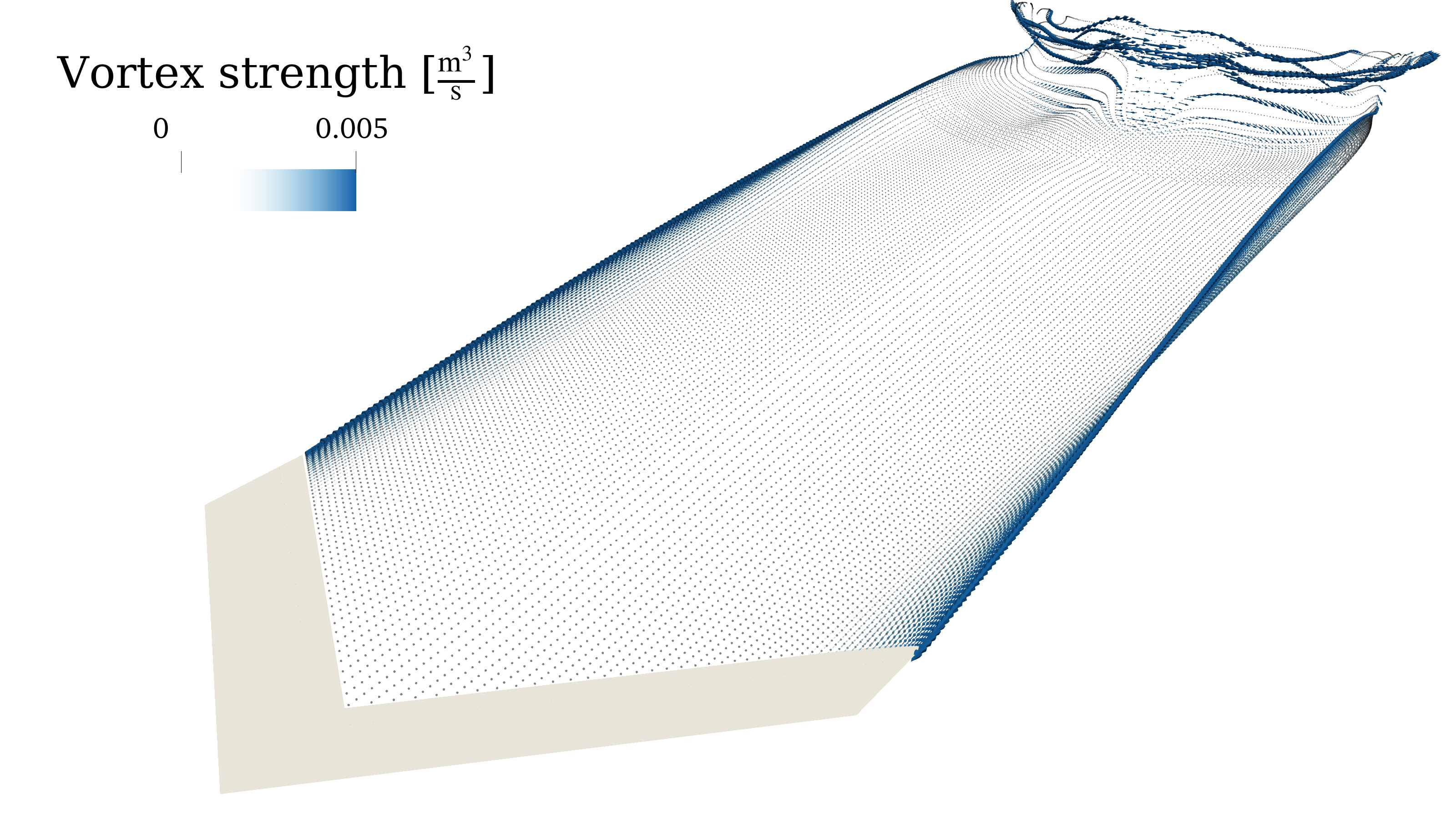
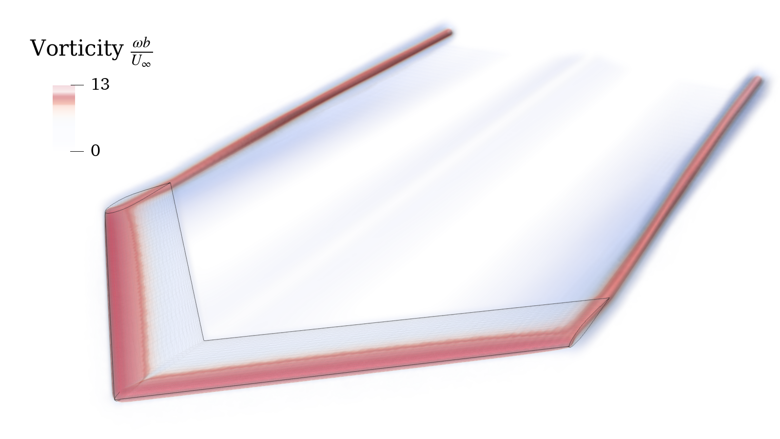
45° swept-back wing at an angle of attack of 4.2°. This wing has an aspect
ratio of 5.0, a RAE 101 airfoil section with 12% thickness, and no dihedral,
twist, nor taper. This test case matches the experimental setup of Weber,
J., and Brebner, G., “Low-Speed Tests on 45-deg Swept-Back Wings, Part I,”
Tech. rep., 1951. The same case is used in a VLM calculation in Bertin's
Aerodynamics for Engineers, Example 7.2, pp. 343.
# AUTHORSHIP
* Author : Eduardo J. Alvarez (edoalvarez.com)
* Email : Edo.AlvarezR@gmail.com
* Created : Feb 2023
* Last updated : Feb 2023
* License : MIT
=###############################################################################
import FLOWUnsteady as uns
import FLOWVLM as vlm
run_name = "wing-example" # Name of this simulation
save_path = run_name # Where to save this simulation
paraview = true # Whether to visualize with Paraview
# ----------------- SIMULATION PARAMETERS --------------------------------------
AOA = 4.2 # (deg) angle of attack
magVinf = 49.7 # (m/s) freestream velocity
rho = 0.93 # (kg/m^3) air density
qinf = 0.5*rho*magVinf^2 # (Pa) static pressure
Vinf(X, t) = magVinf*[cosd(AOA), 0.0, sind(AOA)] # Freestream function
# ----------------- GEOMETRY PARAMETERS ----------------------------------------
b = 2.489 # (m) span length
ar = 5.0 # Aspect ratio b/c_tip
tr = 1.0 # Taper ratio c_tip/c_root
twist_root = 0.0 # (deg) twist at root
twist_tip = 0.0 # (deg) twist at tip
lambda = 45.0 # (deg) sweep
gamma = 0.0 # (deg) dihedral
# Discretization
n = 50 # Number of spanwise elements per side
r = 10.0 # Geometric expansion of elements
central = false # Whether expansion is central
# NOTE: A geometric expansion of 10 that is not central means that the last
# element is 10 times wider than the first element. If central, the
# middle element is 10 times wider than the peripheral elements.
# ----------------- SOLVER PARAMETERS ------------------------------------------
# Time parameters
wakelength = 2.75*b # (m) length of wake to be resolved
ttot = wakelength/magVinf # (s) total simulation time
nsteps = 200 # Number of time steps
# VLM and VPM parameters
p_per_step = 1 # Number of particle sheds per time step
lambda_vpm = 2.0 # VPM core overlap
sigma_vpm_overwrite = lambda_vpm * magVinf * (ttot/nsteps)/p_per_step # Smoothing core size
sigma_vlm_solver= -1 # VLM-on-VLM smoothing radius (deactivated with <0)
sigma_vlm_surf = 0.05*b # VLM-on-VPM smoothing radius
shed_starting = true # Whether to shed starting vortex
vlm_rlx = 0.7 # VLM relaxation
# ----------------- 1) VEHICLE DEFINITION --------------------------------------
println("Generating geometry...")
# Generate wing
wing = vlm.simpleWing(b, ar, tr, twist_root, lambda, gamma;
twist_tip=twist_tip, n=n, r=r, central=central);
# NOTE: `FLOWVLM.simpleWing` is an auxiliary function in FLOWVLM for creating a
# VLM wing with constant sweep, dihedral, and taper ratio, and a linear
# twist between the root and the wing tips
println("Generating vehicle...")
# Generate vehicle
system = vlm.WingSystem() # System of all FLOWVLM objects
vlm.addwing(system, "Wing", wing)
vlm_system = system; # System solved through VLM solver
wake_system = system; # System that will shed a VPM wake
vehicle = uns.VLMVehicle( system;
vlm_system=vlm_system,
wake_system=wake_system
);
# NOTE: `FLOWUnsteady.VLMVehicle` creates a vehicle made out of multiple VLM and
# rotor subsystems. The argument `system` represents the vehicle as a
# whole which will be translated and rotated with the kinematics
# prescribed by the maneuver. The subsystem `vlm_system` will be solved
# with the VLM solver. The subsystems `rotor_systems` are solved with
# blade elements (none in this case). The subsystem `wake_system` will
# shed the VPM wake.
# ------------- 2) MANEUVER DEFINITION -----------------------------------------
Vvehicle(t) = zeros(3) # Translational velocity of vehicle over time
anglevehicle(t) = zeros(3) # Angle of the vehicle over time
angle = () # Angle of each tilting system (none)
RPM = () # RPM of each rotor system (none)
maneuver = uns.KinematicManeuver(angle, RPM, Vvehicle, anglevehicle)
# NOTE: `FLOWUnsteady.KinematicManeuver` defines a maneuver with prescribed
# kinematics. `Vvehicle` defines the velocity of the vehicle (a vector)
# over time. `anglevehicle` defines the attitude of the vehicle over time
# (a vector with inclination angles with respect to each axis of the
# global coordinate system). `angle` defines the tilting angle of each
# tilting system over time (none in this case). `RPM` defines the RPM of
# each rotor system over time (none in this case).
# Each of these functions receives a nondimensional time `t`, which is the
# simulation time normalized by the total time `ttot`, from 0 to
# 1, beginning to end of simulation. They all return a nondimensional
# output that is then scaled up by either a reference velocity (`Vref`) or
# a reference RPM (`RPMref`). Defining the kinematics and controls of the
# maneuver in this way allows the user to have more control over how fast
# to perform the maneuver, since the total time, reference velocity and
# RPM are then defined in the simulation parameters shown below.
# ------------- 3) SIMULATION DEFINITION ---------------------------------------
Vref = 0.0 # Reference velocity to scale maneuver by
RPMref = 0.0 # Reference RPM to scale maneuver by
Vinit = Vref*Vvehicle(0) # Initial vehicle velocity
Winit = pi/180*(anglevehicle(1e-6) - anglevehicle(0))/(1e-6*ttot) # Initial angular velocity
# Maximum number of particles
max_particles = (nsteps+1)*(vlm.get_m(vehicle.vlm_system)*(p_per_step+1) + p_per_step)
simulation = uns.Simulation(vehicle, maneuver, Vref, RPMref, ttot;
Vinit=Vinit, Winit=Winit);
# ------------- 4) MONITORS DEFINITIONS ----------------------------------------
# NOTE: Monitors are functions that are called at every time step to perform
# some secondary computation after the solution of that time step has been
# obtained. In this case, the wing monitor uses the circulation and
# induced velocities to compute aerodynamic forces and decompose them
# into lift and drag. The monitor then plots these forces at every time
# step while also saving them under a CSV file in the simulation folder.
# Generate function that calculates aerodynamic forces
# NOTE: We exclude skin friction since we want to compare to the experimental
# data reported in Weber 1951 that was measured with pressure taps
calc_aerodynamicforce_fun = uns.generate_calc_aerodynamicforce(;
add_parasiticdrag=true,
add_skinfriction=false,
airfoilpolar="xf-rae101-il-1000000.csv"
)
D_dir = [cosd(AOA), 0.0, sind(AOA)] # Direction of drag
L_dir = uns.cross(D_dir, [0,1,0]) # Direction of lift
figs, figaxs = [], [] # Figures generated by monitor
# Generate wing monitor
monitor_wing = uns.generate_monitor_wing(wing, Vinf, b, ar,
rho, qinf, nsteps;
calc_aerodynamicforce_fun=calc_aerodynamicforce_fun,
L_dir=L_dir,
D_dir=D_dir,
out_figs=figs,
out_figaxs=figaxs,
save_path=save_path,
run_name=run_name,
figname="wing monitor",
);
# ------------- 5) RUN SIMULATION ----------------------------------------------
println("Running simulation...")
uns.run_simulation(simulation, nsteps;
# ----- SIMULATION OPTIONS -------------
Vinf=Vinf,
rho=rho,
# ----- SOLVERS OPTIONS ----------------
p_per_step=p_per_step,
max_particles=max_particles,
sigma_vlm_solver=sigma_vlm_solver,
sigma_vlm_surf=sigma_vlm_surf,
sigma_rotor_surf=sigma_vlm_surf,
sigma_vpm_overwrite=sigma_vpm_overwrite,
shed_starting=shed_starting,
vlm_rlx=vlm_rlx,
extra_runtime_function=monitor_wing,
# ----- OUTPUT OPTIONS ------------------
save_path=save_path,
run_name=run_name
);
# ----------------- 6) VISUALIZATION -------------------------------------------
if paraview
println("Calling Paraview...")
# Files to open in Paraview
files = joinpath(save_path, run_name*"_Wing_vlm...vtk")
files *= ";"*run_name*"_pfield...xmf;"
# Call Paraview
run(`paraview --data=$(files)`)
end
Reduce resolution (n and steps) to speed up simulation without loss of accuracy.
As the simulation runs, you will see the monitor (shown below) plotting the lift and drag coefficients over time along with the loading distribution. For comparison, here we have also added the experimental measurements reported by Weber and Brebner, 1951.
(red = beginning, blue = end)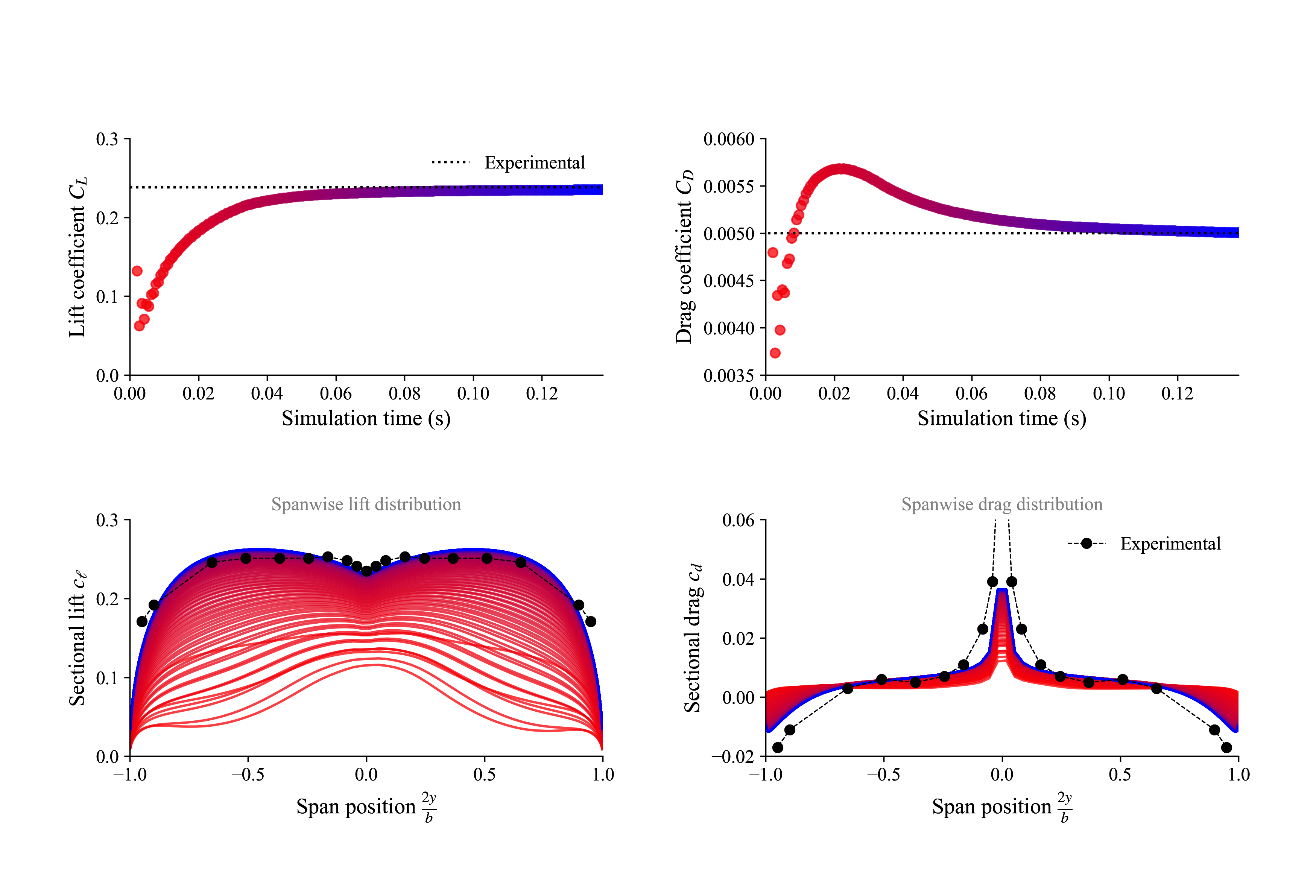
| Experimental | FLOWUnsteady | Error | |
|---|---|---|---|
| $C_L$ | 0.238 | 0.23506 | 1.234% |
| $C_D$ | 0.005 | 0.00501 | 0.143% |
The .pvsm file visualizing the simulation as shown at the top of this page is available here: LINK (right click → save as...). To open in Paraview: File → Load State → (select .pvsm file) then select "Search files under specified directory" and point it to the folder where the simulation was saved.