Incidence Sweep

In simple cases like a propeller in cruise, steady and quasi-steady methods like blade element momentum theory can be as accurate as a fully unsteady simulation, and even faster. However, in more complex cases, quasi-steady solvers are far from accurate and a fully unsteady solver is needed. We now highlight one of such cases: the case of a propeller at an incidence angle.

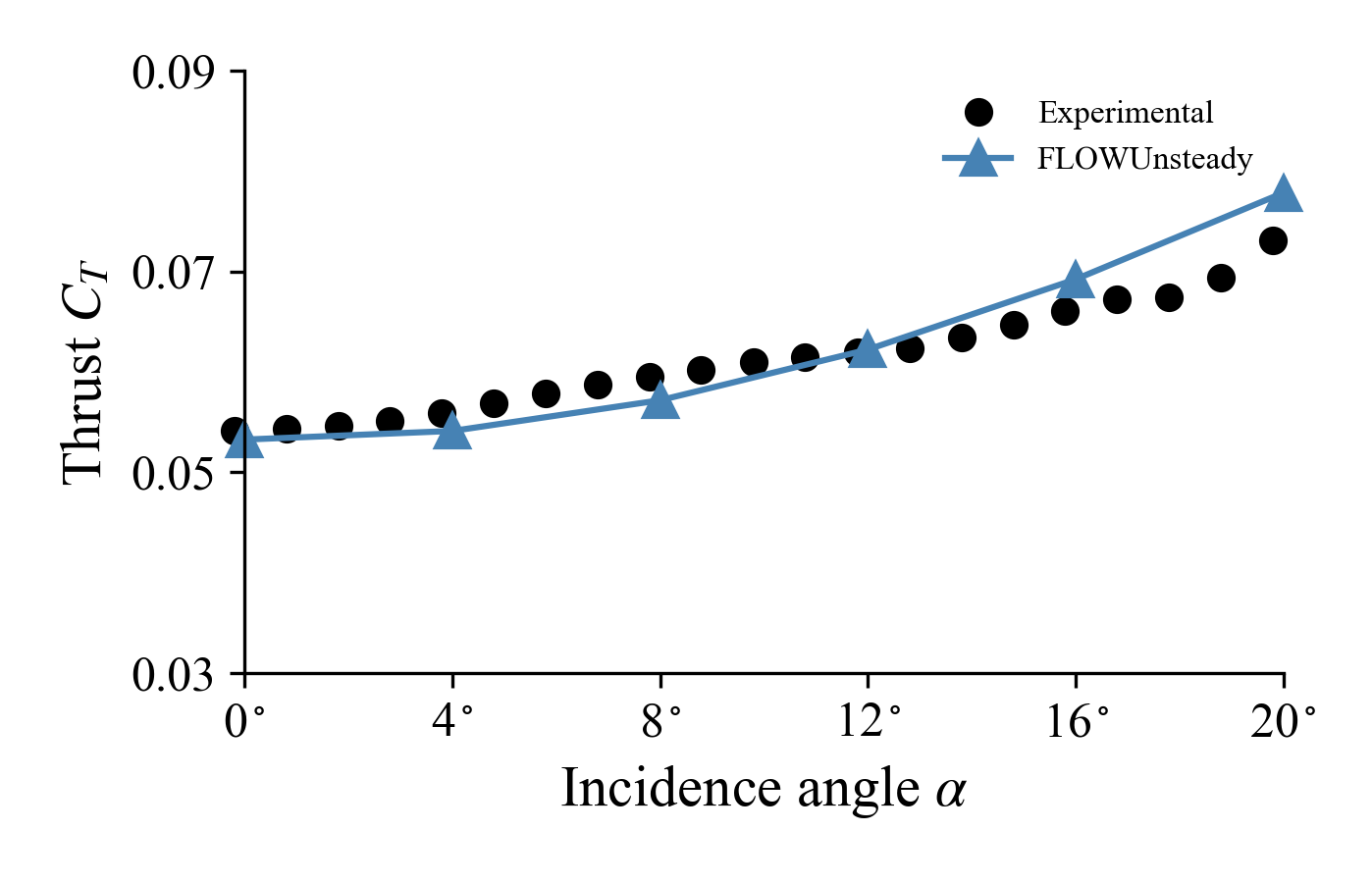
A rotor operating at an incidence angle relative to the freestream experiences an unsteady loading due to the blade seeing a larger local velocity in the advancing side of the rotor and a smaller local velocity in the retreating side. This also causes a wake that is skewed. For this example we will run a sweep of simulations on a 4-bladed propeller operating at multiple incidence angles $\alpha$ (where $\alpha=0^\circ$ is fully axial inflow, and $\alpha=90^\circ$ is fully edgewise inflow).

#=##############################################################################
# DESCRIPTION
    Simulation of Beaver propeller (four-bladed rotor, 9.34-inch diameter) at
    various incidence angles.

    This example uses the blade geometry reported in Sinnige & de Vries (2018),
    "Unsteady Pylon Loading Caused by Propeller-Slipstream Impingement for
    Tip-Mounted Propellers," and replicates the experiment conducted by Sinnige
    et al. (2019), "Wingtip-Mounted Propellers: Aerodynamic Analysis of
    Interaction Effects and Comparison with Conventional Layout."

# AUTHORSHIP
  * Author          : Eduardo J. Alvarez (edoalvarez.com)
  * Email           : Edo.AlvarezR@gmail.com
  * Created         : Mar 2023
  * Last updated    : Mar 2023
  * License         : MIT
=###############################################################################

import FLOWUnsteady as uns
import FLOWVLM as vlm

case_name       = "propeller-incidencesweep-example"    # Name of this sweep case

save_path       = case_name                 # Where to save this sweep
output_runs     = [20]                      # Saves the VTK output of these AOAs for viz


# ----------------- GEOMETRY PARAMETERS ----------------------------------------

# Rotor geometry
rotor_file      = "beaver.csv"              # Rotor geometry
data_path       = uns.def_data_path         # Path to rotor database
pitch           = 0.0                       # (deg) collective pitch of blades
CW              = false                     # Clock-wise rotation
xfoil           = false                     # Whether to run XFOIL
read_polar      = vlm.ap.read_polar2        # What polar reader to use

# Discretization
n               = 20                        # Number of blade elements per blade
r               = 1/5                       # Geometric expansion of elements

# Read radius of this rotor and number of blades
R, B            = uns.read_rotor(rotor_file; data_path=data_path)[[1,3]]

# ----------------- SIMULATION PARAMETERS --------------------------------------

# Operating conditions
AOAs            = 0:4:20                    # (deg) incidence angles to evaluate
magVinf         = 40.0                      # (m/s) freestream velocity
J               = 0.9                       # Advance ratio Vinf/(nD)
RPM             = magVinf / (2*R/60) / J    # RPM

rho             = 1.225                     # (kg/m^3) air density
mu              = 1.79e-5                   # (kg/ms) air dynamic viscosity
speedofsound    = 342.35                    # (m/s) speed of sound


ReD             = 2*pi*RPM/60*R * rho/mu * 2*R      # Diameter-based Reynolds number
Matip           = 2*pi*RPM/60*R / speedofsound      # Tip Mach number

println("""
    RPM:    $(RPM)
    Vinf:   $(magVinf) m/s
    Matip:  $(round(Matip, digits=3))
    ReD:    $(round(ReD, digits=0))
""")

# ----------------- SOLVER PARAMETERS ------------------------------------------

# Aerodynamic solver
VehicleType     = uns.UVLMVehicle           # Unsteady solver

# Time parameters
nrevs           = 4                         # Number of revolutions in simulation
nsteps_per_rev  = 36                        # Time steps per revolution
nsteps          = nrevs*nsteps_per_rev      # Number of time steps
ttot            = nsteps/nsteps_per_rev / (RPM/60)       # (s) total simulation time

# VPM particle shedding
p_per_step      = 2                         # Sheds per time step
shed_starting   = true                      # Whether to shed starting vortex
shed_unsteady   = true                      # Whether to shed vorticity from unsteady loading
max_particles   = ((2*n+1)*B)*nsteps*p_per_step + 1 # Maximum number of particles

# Regularization
sigma_rotor_surf= R/40                      # Rotor-on-VPM smoothing radius
# sigma_rotor_surf= R/80
lambda_vpm      = 2.125                     # VPM core overlap
                                            # VPM smoothing radius
sigma_vpm_overwrite = lambda_vpm * 2*pi*R/(nsteps_per_rev*p_per_step)

# Rotor solver
vlm_rlx         = 0.7                       # VLM relaxation <-- this also applied to rotors
                                            # Prandtl's tip correction with a strong hub
hubtiploss_correction = ( (0.75, 10, 0.5, 0.05), (1, 1, 1, 1.0) ) # correction up to r/R = 0.35

if VehicleType == uns.QVLMVehicle           # Mute colinear warnings if quasi-steady solver
    uns.vlm.VLMSolver._mute_warning(true)
end


# ----------------- 1) VEHICLE DEFINITION --------------------------------------
println("Generating geometry...")

# Generate rotor
rotor = uns.generate_rotor(rotor_file; pitch=pitch,
                                        n=n, CW=CW, blade_r=r,
                                        altReD=[RPM, J, mu/rho],
                                        xfoil=xfoil,
                                        read_polar=read_polar,
                                        data_path=data_path,
                                        verbose=true,
                                        verbose_xfoil=false,
                                        plot_disc=true
                                        );

println("Generating vehicle...")

# Generate vehicle
system = vlm.WingSystem()                   # System of all FLOWVLM objects
vlm.addwing(system, "Rotor", rotor)

rotors = [rotor];                           # Defining this rotor as its own system
rotor_systems = (rotors, );                 # All systems of rotors

wake_system = vlm.WingSystem()              # System that will shed a VPM wake
                                            # NOTE: Do NOT include rotor when using the quasi-steady solver
if VehicleType != uns.QVLMVehicle
    vlm.addwing(wake_system, "Rotor", rotor)
end

vehicle = VehicleType(   system;
                            rotor_systems=rotor_systems,
                            wake_system=wake_system
                         );


# ------------- 2) MANEUVER DEFINITION -----------------------------------------
# Non-dimensional translational velocity of vehicle over time
Vvehicle(t) = zeros(3)

# Angle of the vehicle over time
anglevehicle(t) = zeros(3)

# RPM control input over time (RPM over `RPMref`)
RPMcontrol(t) = 1.0

angles = ()                                 # Angle of each tilting system (none)
RPMs = (RPMcontrol, )                       # RPM of each rotor system

maneuver = uns.KinematicManeuver(angles, RPMs, Vvehicle, anglevehicle)


# ------------- 3) SIMULATION DEFINITION ---------------------------------------

Vref = 0.0                                  # Reference velocity to scale maneuver by
RPMref = RPM                                # Reference RPM to scale maneuver by

Vinit = Vref*Vvehicle(0)                    # Initial vehicle velocity
Winit = pi/180*(anglevehicle(1e-6) - anglevehicle(0))/(1e-6*ttot)  # Initial angular velocity

simulation = uns.Simulation(vehicle, maneuver, Vref, RPMref, ttot;
                                                    Vinit=Vinit, Winit=Winit);

# ------------- RUN AOA SWEEP --------------------------------------------------

# Create path where to save sweep
uns.gt.create_path(save_path, true)

for AOA in AOAs

    println("\n\nRunning AOA = $(AOA)")

    Vinf(X, t)      = magVinf*[cosd(AOA), sind(AOA), 0] # (m/s) freestream velocity vector

    # ------------- 4) MONITOR DEFINITION ---------
    monitor_rotor = uns.generate_monitor_rotors(rotors, J, rho, RPM, nsteps;
                                                t_scale=RPM/60,
                                                t_lbl="Revolutions",
                                                save_path=save_path,
                                                run_name="AOA$(ceil(Int, AOA*100))",
                                                disp_conv=false
                                                )

    # ------------- 5) RUN SIMULATION -------------
    println("\tRunning simulation...")

    save_vtks = AOA in output_runs ? save_path*"-AOA$(ceil(Int, AOA*100))" : nothing

    uns.run_simulation(simulation, nsteps;
                        # ----- SIMULATION OPTIONS -------------
                        Vinf=Vinf,
                        rho=rho, mu=mu, sound_spd=speedofsound,
                        # ----- SOLVERS OPTIONS ----------------
                        p_per_step=p_per_step,
                        max_particles=max_particles,
                        sigma_vlm_surf=sigma_rotor_surf,
                        sigma_rotor_surf=sigma_rotor_surf,
                        sigma_vpm_overwrite=sigma_vpm_overwrite,
                        vlm_rlx=vlm_rlx,
                        hubtiploss_correction=hubtiploss_correction,
                        shed_unsteady=shed_unsteady,
                        shed_starting=shed_starting,
                        extra_runtime_function=monitor_rotor,
                        # ----- OUTPUT OPTIONS ------------------
                        save_path=save_vtks,
                        run_name="singlerotor",
                        v_lvl=1, verbose_nsteps=24
                        );
end

Check examples/propeller/propeller_incidence.jl to postprocess and plot the results as shown below.