(4) Monitors Definitions
A monitor is a function that is passed to FLOWUnsteady.run_simulation as an extra runtime function that is called at every time step. Runtime functions are expected to return a Boolean that indicates the need of stopping the simulation, such that if extra_runtime_function ever returns true, the simulation will immediately be ended.
Multiple monitors can be concatenated with boolean logic as follows
import FLOWUnsteady as uns

monitor_states = uns.generate_monitor_statevariables()
monitor_enstrophy = uns.generate_monitor_enstrophy()

monitors(args...; optargs...) = monitor_states(args...; optargs...) || monitor_enstrophy(args...; optargs...)
Then pass the monitor to the simulation as
uns.run_simulation(sim, nsteps; extra_runtime_function=monitors, ...)FLOWUnsteady facilitates the concatenation of monitors through the function FLOWUnsteady.concatenate. Using this function, the example above looks like this:
monitor_states = uns.generate_monitor_statevariables()
monitor_enstrophy = uns.generate_monitor_enstrophy()

allmonitors = [monitor_states, monitor_enstrophy]

monitors = uns.concatenate(monitors)

uns.run_simulation(sim, nsteps; extra_runtime_function=monitors, ...)
Monitor Generators
The following are functions for generating the monitors that serve most use cases. See the source code of these monitors to get an idea of how to write your own user-defined monitors.
FLOWUnsteady.generate_monitor_statevariables — Functiongenerate_monitor_statevariables(; save_path=nothing)Generate a monitor plotting the state variables of the vehicle at every time step. The state variables are vehicle velocity, vehicle angular velocity, and vehicle position.
Use save_path to indicate a directory where to save the plots.
Here is an example of this monitor on a vehicle flying a circular path: 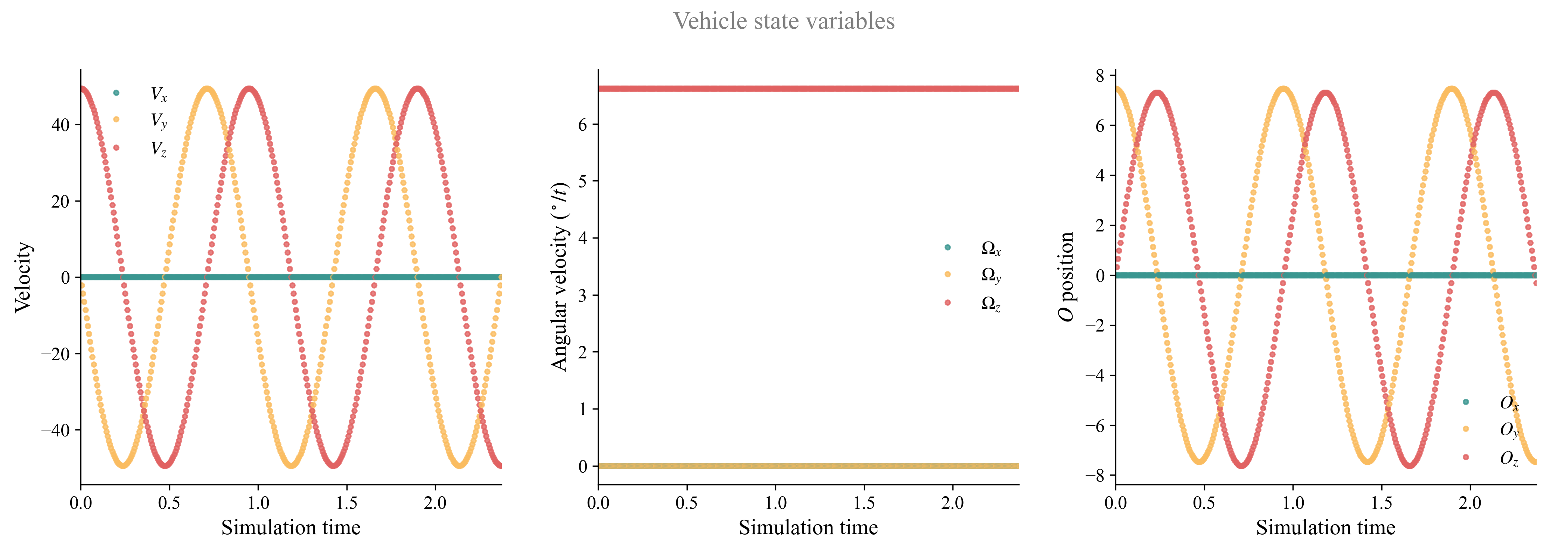
FLOWUnsteady.generate_monitor_wing — Functiongenerate_monitor_wing(wing::Union{vlm.Wing, vlm.WingSystem},
Vinf::Function, b_ref::Real, ar_ref::Real,
rho_ref::Real, qinf_ref::Real, nsteps_sim::Int;
L_dir=[0,0,1], # Direction of lift component
D_dir=[1,0,0], # Direction of drag component
calc_aerodynamicforce_fun=FLOWUnsteady.generate_calc_aerodynamicforce())Generate a wing monitor computing and plotting the aerodynamic force and wing loading at every time step.
The aerodynamic force is integrated, decomposed, and reported as overall lift coefficient $C_L = \frac{L}{\frac{1}{2}\rho u_\infty^2 b c}$ and drag coefficient ${C_D = \frac{D}{\frac{1}{2}\rho u_\infty^2 b c}}$. The wing loading is reported as the sectional lift and drag coefficients defined as $c_\ell = \frac{\ell}{\frac{1}{2}\rho u_\infty^2 c}$ and $c_d = \frac{d}{\frac{1}{2}\rho u_\infty^2 c}$, respectively.
The aerodynamic force is calculated through the function calc_aerodynamicforce_fun, which is a user-defined function. The function can also be automatically generated through, generate_calc_aerodynamicforce which defaults to incluiding the Kutta-Joukowski force, parasitic drag (calculated from a NACA 0012 airfoil polar), and unsteady-circulation force.
b_ref: Reference span length.ar_ref: Reference aspect ratio, used to calculate the equivalent chord $c = \frac{b}{\mathrm{ar}}$.rho_ref: Reference density.qinf_ref: Reference dynamic pressure $q_\infty = \frac{1}{2}\rho u_\infty^2$.nsteps_sim: the number of time steps by the end of the simulation (used for generating the color gradient).- Use
save_pathto indicate a directory where to save the plots. If so, it will also generate a CSV file with $C_L$ and $C_D$.
Here is an example of this monitor: 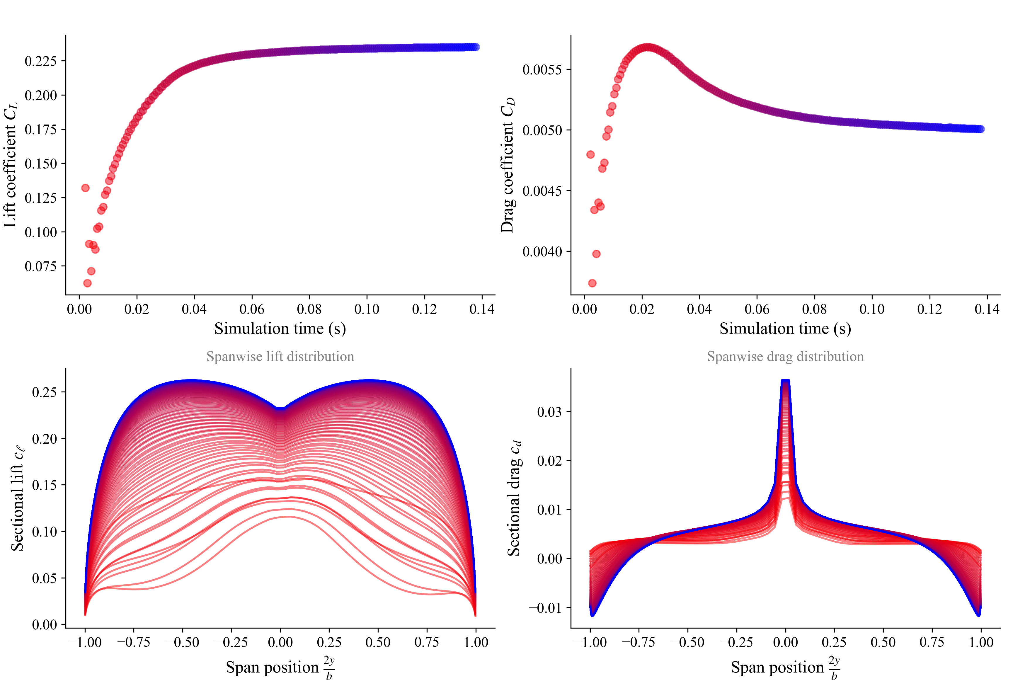
FLOWUnsteady.generate_monitor_rotors — Functiongenerate_monitor_rotors(rotors::Array{vlm.Rotor}, J_ref::Real,
rho_ref::Real, RPM_ref::Real, nsteps_sim::Int;
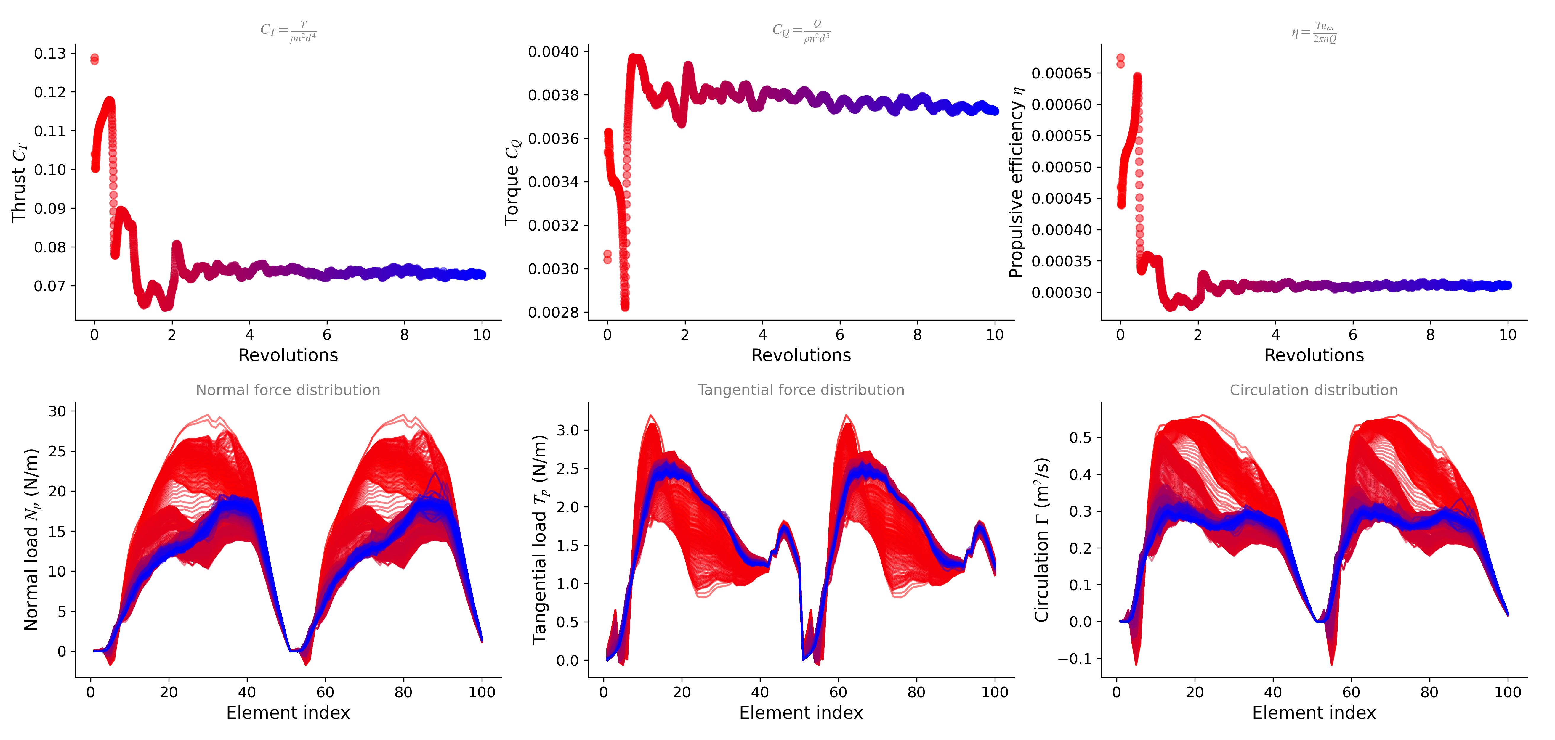
save_path=nothing)Generate a rotor monitor plotting the aerodynamic performance and blade loading at every time step.
The aerodynamic performance consists of thrust coefficient $C_T=\frac{T}{\rho n^2 d^4}$, torque coefficient $C_Q = \frac{Q}{\rho n^2 d^5}$, and propulsive efficiency $\eta = \frac{T u_\infty}{2\pi n Q}$.
J_refandrho_refare the reference advance ratio and air density used for calculating propulsive efficiency and coefficients. The advance ratio used here is defined as $J=\frac{u_\infty}{n d}$ with $n = \frac{\mathrm{RPM}}{60}$.RPM_refis the reference RPM used to estimate the age of the wake.nsteps_simis the number of time steps by the end of the simulation (used for generating the color gradient).- Use
save_pathto indicate a directory where to save the plots. If so, it will also generate a CSV file with $C_T$, $C_Q$, and $\eta$.
FLOWUnsteady.generate_monitor_enstrophy — Functiongenerate_monitor_enstrophy(; save_path=nothing)Generate a monitor plotting the global enstrophy of the flow at every time step (computed through the particle field). This is calculated by integrating the local enstrophy defined as ξ = ω⋅ω / 2.
Enstrophy is approximated as 0.5*Σ( Γ𝑝⋅ω(x𝑝) ). This is consistent with Winckelamns' 1995 CTR report, "Some Progress in LES using the 3-D VPM".
Use save_path to indicate a directory where to save the plots. If so, it will also generate a CSV file with ξ.
Here is an example of this monitor: 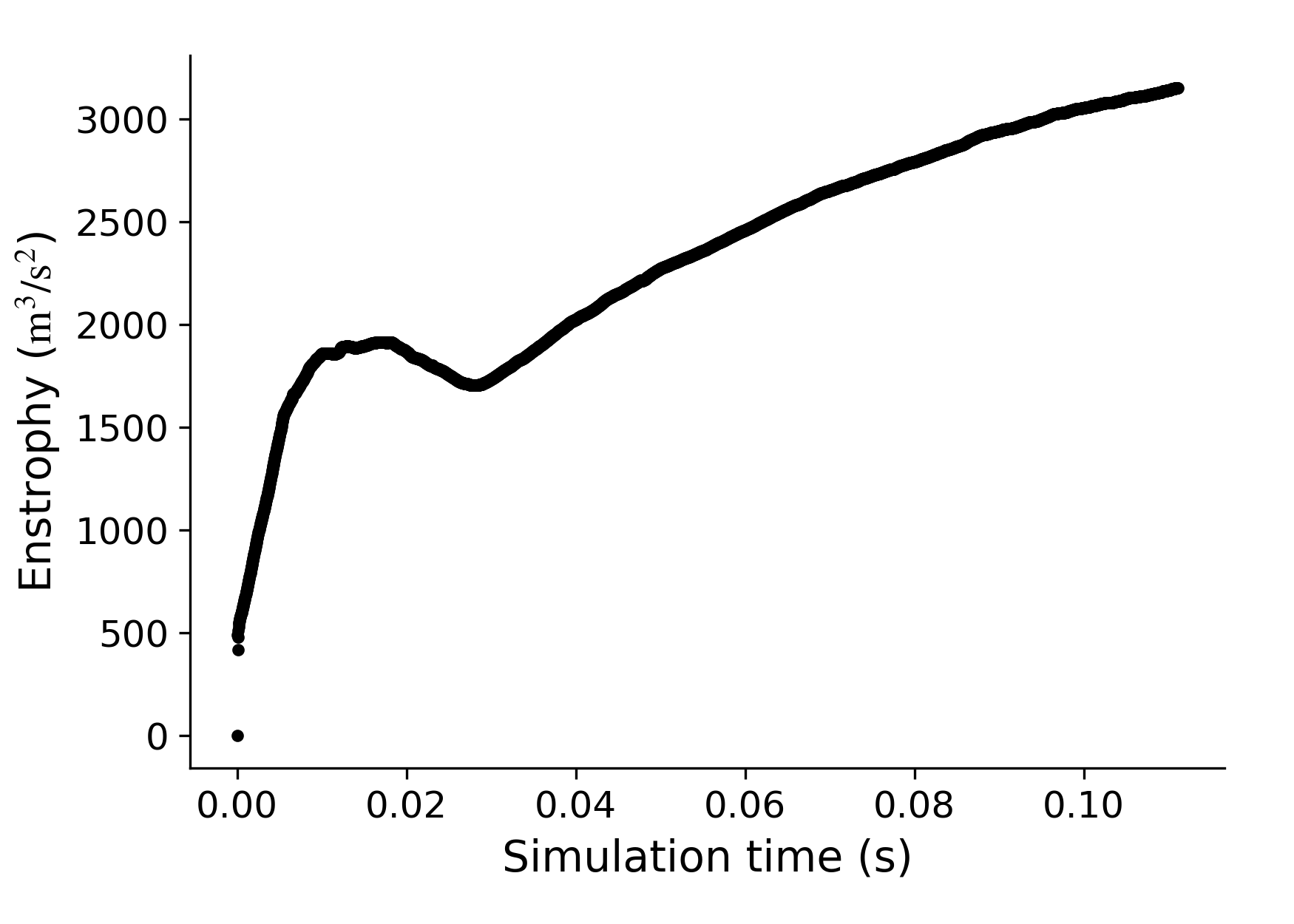
FLOWUnsteady.generate_monitor_Cd — Functiongenerate_monitor_Cd(; save_path=nothing)Generate a monitor plotting the mean value of the SFS model coefficient $C_d$ across the particle field at every time step. It also plots the ratio of $C_d$ values that were clipped to zero (not included in the mean).
Use save_path to indicate a directory where to save the plots. If so, it will also generate a CSV file with the statistics of $C_d$ (particles whose coefficients have been clipped are ignored).
Here is an example of this monitor: 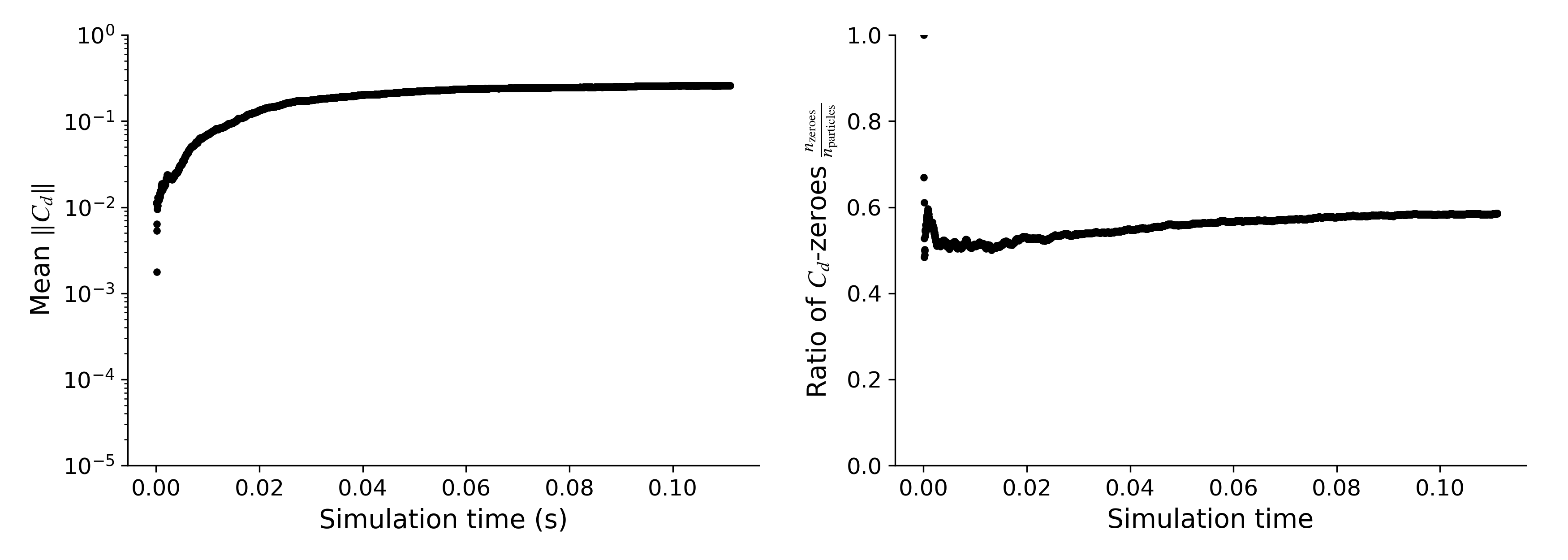
FLOWUnsteady.concatenate — Functionconcatenate(monitors::Array{Function})
concatenate(monitors::NTuple{N, Function})
concatenate(monitor1, monitor2, ...)Concatenates a collection of monitors into a pipeline, returning one monitor of the form
monitor(args...; optargs...) =
monitors[1](args...; optargs...) || monitors[2](args...; optargs...) || ...Force Calculators
The following are some possible methods for calculating aerodynamic forces. Generator functions return a function that can be directly passed to FLOWUnsteady.generate_monitor_wing through the keyword argument calc_aerodynamicforce_fun.
FLOWUnsteady.generate_calc_aerodynamicforce — Functiongenerate_calc_aerodynamicforce(; add_parasiticdrag=false,
add_skinfriction=true,
airfoilpolar="xf-n0012-il-500000-n5.csv",
parasiticdrag_args=(),
)Default method for calculating aerodynamic forces.
Pass the output of this function to generate_monitor_wing, or use this as an example on how to define your own costumized force calculations.
This function stitches together the outputs of generate_aerodynamicforce_kuttajoukowski and generate_aerodynamicforce_parasiticdrag, and calc_aerodynamicforce_unsteady. See Alvarez' dissertation, Sec. 6.3.3.
FLOWUnsteady.generate_aerodynamicforce_kuttajoukowski — Functiongenerate_aerodynamicforce_kuttajoukowski(KJforce_type::String,
sigma_vlm_surf, sigma_rotor_surf,
vlm_vortexsheet,
vlm_vortexsheet_overlap,
vlm_vortexsheet_distribution,
vlm_vortexsheet_sigma_tbv;
vehicle=nothing
)Calculates the aerodynamic force at each element of a VLM system using its current Gamma solution and the Kutta-Joukowski theorem. It saves the force as the field vlm_system.sol["Ftot"]
This force calculated through the Kutta-Joukowski theorem uses the freestream velocity, kinematic velocity, and wake-induced velocity on each bound vortex. See Alvarez' dissertation, Sec. 6.3.3.
ARGUMENTS
vlm_vortexsheet::Bool: If true, the bound vorticity is approximated with and actuator surface model through a vortex sheet. If false, it is approximated with an actuator line model with horseshoe vortex filaments.vlm_vortexsheet_overlap::Bool: Target core overlap between particles representing the vortex sheet (ifvlm_vortexsheet=true).vlm_vortexsheet_distribution::Function: Vorticity distribution in vortex sheet (seeg_uniform,g_linear, andg_pressure).KJforce_type::String: Ifvlm_vortexsheet=true, it specifies how to weight the force of each particle in the vortex sheet. IfKJforce_type=="averaged", the KJ force is a chordwise average of the force experienced by the particles. IfKJforce_type=="weighted", the KJ force is chordwise weighted by the strength of each particle. IfKJforce_type=="regular", the vortex sheet is ignored, and the KJ force is calculated from the velocity induced at midpoint between the horseshoe filaments.vehicle::VLMVehicle: Ifvlm_vortexsheet=true, it is expected that the vehicle object is passed through this argument.
FLOWUnsteady.generate_aerodynamicforce_parasiticdrag — Functiongenerate_aerodynamicforce_parasiticdrag(polar_file::String;
read_path=FLOWUnsteady.default_database*"/airfoils",
calc_cd_from_cl=false,
add_skinfriction=true,
Mach=nothing)Calculates the parasitic drag along the wing using a lookup airfoil table. It adds this force to the field vlm_system.sol["Ftot"].
The lookup table is read from the file polar_file under the directory read_path. The parasitic drag includes form drag, skin friction, and wave drag, assuming that each of these components are included in the lookup polar. polar_file can be any polar file downloaded from airfoiltools.com.
To ignore skin friction drag, use add_skinfriction=false.
The drag will be calculated from the local effective angle of attack, unless calc_cd_from_cl=true is used, which then will be calculated from the local lift coefficient given by the circulation distribution. cd from cl tends to be more accurate than from AOA, but the method might fail to correlate cd and cl depending on how noise the polar data is.
If Mach != nothing, it will use a Prandtl-Glauert correction to pre-correct the lookup cl. This will have no effects if calc_cd_from_cl=false.
FLOWUnsteady.calc_aerodynamicforce_unsteady — Functioncalc_aerodynamicforce_unsteady(vlm_system::Union{vlm.Wing, vlm.WingSystem},
prev_vlm_system, pfield, Vinf, dt, rho; t=0.0,
per_unit_span=false, spandir=[0, 1, 0],
include_trailingboundvortex=false,
add_to_Ftot=false
)Force from unsteady circulation.
This force tends to add a lot of numerical noise, which in most cases ends up cancelling out when the loading is time-averaged. Hence, add_to_Ftot=false will calculate the unsteady loading and save it under the field Funs-vector, but it will not be added to the Ftot vector that is used to calculate the wing's overall aerodynamic force.
Wake Treatment
Since the full set of state variables is passed to extra_runtime_function, this function can also be used to alter the simulation on the fly. In some circumstances it is desirable to be able to remove or modify particles, which process we call "wake treatment." Wake treatment is often used to reduce computational cost (for instance, by removing particle in regions of the flow that are not of interest), and it can also be used to force numerical stability (for instance, by removing or clipping particles with vortex strengths that grow beyond certain threshold).
These wake treatment methods can be added into the pipeline of extra_runtime_function as follows:
import FLOWUnsteady as uns

# Define monitors
monitor_states = uns.generate_monitor_statevariables()
monitor_enstrophy = uns.generate_monitor_enstrophy()

# Monitor pipeline
monitors = uns.concatenate(monitor_states, monitor_enstrophy)

# Define wake treatment
wake_treatment = uns.remove_particles_sphere(1.0, 1; Xoff=zeros(3))

# Extra runtime function pipeline
extra_runtime_function = uns.concatenate(monitors, wake_treatment)
Then pass this pipeline to the simulation as
uns.run_simulation(sim, nsteps; extra_runtime_function=extra_runtime_function, ...)Below we list a few generator functions that return common wake treatment methods.
FLOWUnsteady.remove_particles_sphere — Functionremove_particles_sphere(Rsphere2, step::Int; Xoff::Vector=zeros(3))Returns an extra_runtime_function that every step steps removes all particles that are outside of a sphere of radius sqrt(Rsphere2) centered around the vehicle or with an offset Xoff from the center of the vehicle.
Use this wake treatment to avoid unnecesary computation by removing particles that have gone beyond the region of interest.
FLOWUnsteady.remove_particles_box — Functionremove_particles_box(Pmin::Vector, Pmax::Vector, step::Int)Returns an extra_runtime_function that every step steps removes all particles that are outside of a box of minimum and maximum vertices Pmin and Pmax.
Use this wake treatment to avoid unnecesary computation by removing particles that have gone beyond the region of interest.
FLOWUnsteady.remove_particles_lowstrength — Functionremove_particles_lowstrength(critGamma2, step)Returns an extra_runtime_function that removes all particles with a vortex strength magnitude that is smaller than sqrt(critGamma2). Use this wake treatment to avoid unnecesary computation by removing particles that have negligibly-low strength.
step indicates every how many steps to remove particles.
FLOWUnsteady.remove_particles_strength — Functionremove_particles_strength(minGamma2, maxGamma2; every_nsteps=1)Returns an extra_runtime_function that removes all particles with a vortex strength magnitude that is larger than sqrt(maxGamma2) or smaller than sqrt(minGamma2). Use every_nsteps to indicate every how many steps to remove particles.
FLOWUnsteady.remove_particles_sigma — Functionremove_particles_sigma(minsigma, maxsigma; every_nsteps=1)Returns an extra_runtime_function that removes all particles with a smoothing radius that is larger than maxsigma or smaller than minsigma. Use every_nsteps to indicate every how many steps to remove particles.