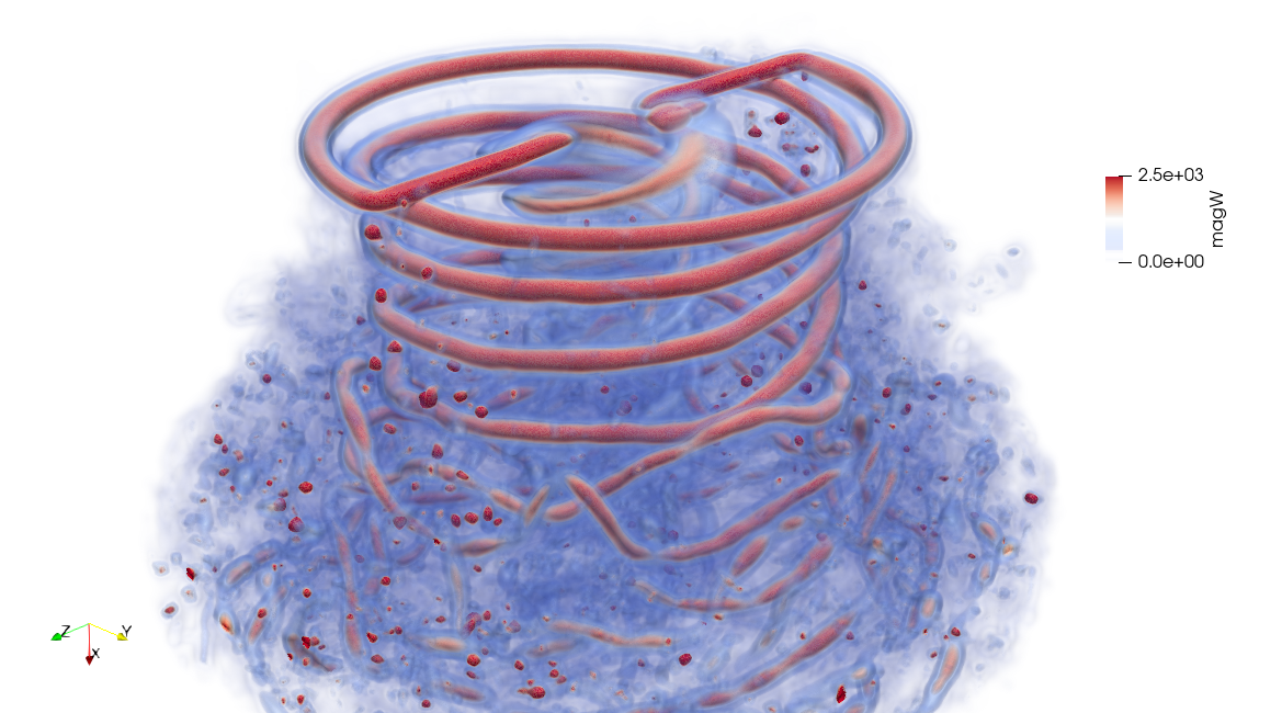
Fluid Domain

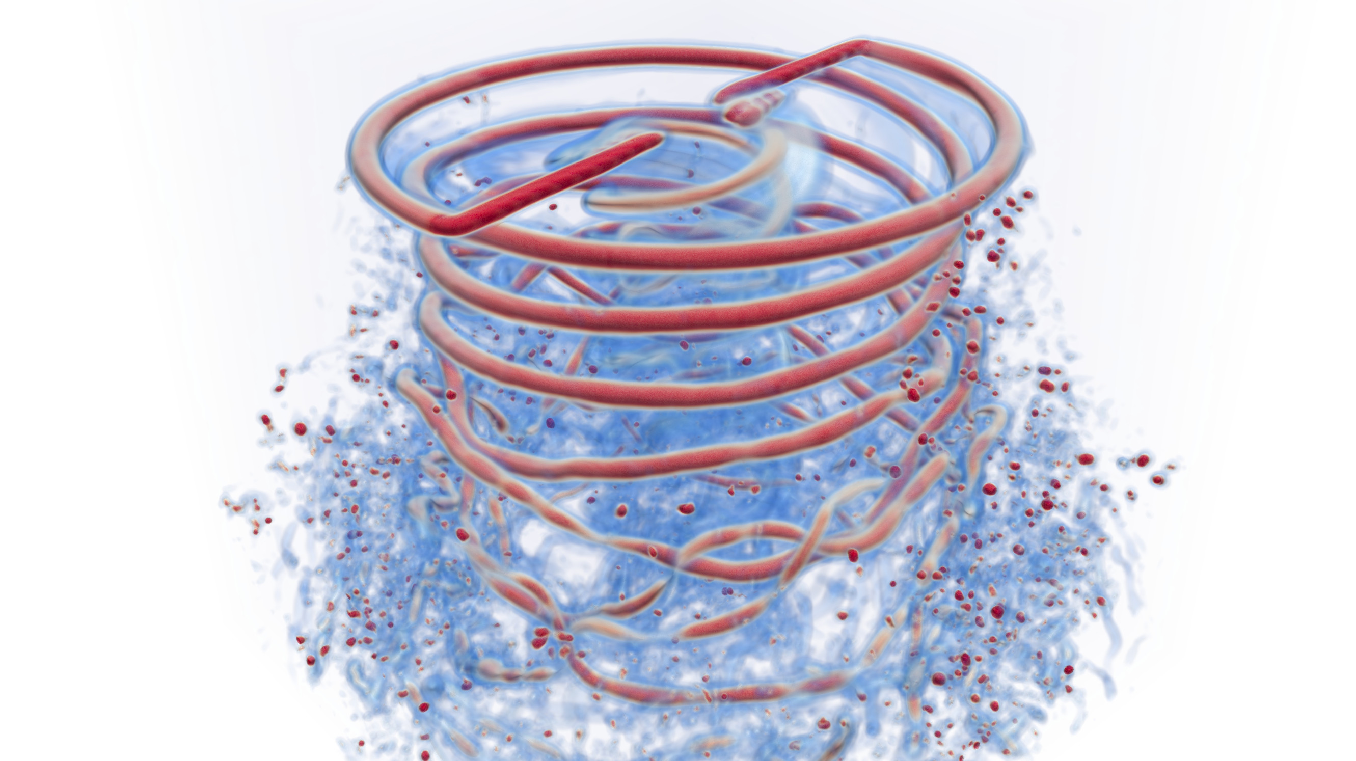
The full fluid domain can be computed in a postprocessing step from the particle field. This is possible because the particle field is a radial basis function that constructs the vorticity field, and the velocity field can be recovered from vorticity through the Biot-Savart law.

Here we show how to use uns.computefluiddomain to read a simulation and process it to generate its fluid domain.

#=##############################################################################
    Computes the fluid domain of DJI 9443 simulation using a volumetric domain.
    This is done probing the velocity and vorticity that the particle field
    induces at each node of a Cartesian grids.

    NOTE: The fluid domain generated here does not include the freestream
            velocity, which needs to be added manually inside ParaView (if any).
=###############################################################################

import FLOWUnsteady as uns
import FLOWUnsteady: vpm, gt, dot, norm

# --------------- INPUTS AND OUTPUTS -------------------------------------------
# INPUT OPTIONS
simulation_name = "rotorhover-example-midhigh00"               # Simulation to read
read_path       = "/home/edoalvar/simulationdata202330/"*simulation_name # Where to read simulation from

pfield_prefix   = "singlerotor_pfield"      # Prefix of particle field files to read
staticpfield_prefix = "singlerotor_staticpfield" # Prefix of static particle field files to read

nums            = [719]              # Time steps to process

# OUTPUT OPTIONS
save_path       = joinpath(read_path, "..", simulation_name*"-fdom")  # Where to save fluid domain
output_prefix   = "singlerotor"             # Prefix of output files
prompt          = true                      # Whether to prompt the user
verbose         = true                      # Enable verbose
v_lvl           = 0                         # Verbose indentation level


# -------------- PARAMETERS ----------------------------------------------------
# Simulation information
R               = 0.12                      # (m) rotor radius
AOA             = 0.0                       # (deg) angle of attack or incidence angle

# Grid
L               = R                         # (m) reference length
dx, dy, dz      = L/50, L/50, L/50          # (m) cell size in each direction
Pmin            = L*[-0.50, -1.25, -1.25]   # (m) minimum bounds
Pmax            = L*[ 2.00,  1.25,  1.25]   # (m) maximum bounds
NDIVS           = ceil.(Int, (Pmax .- Pmin)./[dx, dy, dz])  # Number of cells in each direction
nnodes          = prod(NDIVS .+ 1)          # Total number of nodes

Oaxis           = gt.rotation_matrix2(0, 0, AOA)    # Orientation of grid

# VPM settings
maxparticles    = Int(1.0e6 + nnodes)         # Maximum number of particles
fmm             = vpm.FMM(; p=4, ncrit=50, theta=0.4, phi=0.3) # FMM parameters (decrease phi to reduce FMM noise)
scale_sigma     = 1.00                      # Shrink smoothing radii by this factor
f_sigma         = 0.5                       # Smoothing of node particles as sigma = f_sigma*meansigma

maxsigma        = L/10                      # Particles larger than this get shrunk to this size (this helps speed up computation)
maxmagGamma     = Inf                       # Any vortex strengths larger than this get clipped to this value

include_staticparticles = true              # Whether to include the static particles embedded in the solid surfaces

other_file_prefs = include_staticparticles ? [staticpfield_prefix] : []
other_read_paths = [read_path for i in 1:length(other_file_prefs)]

if verbose
    println("\t"^(v_lvl)*"Fluid domain grid")
    println("\t"^(v_lvl)*"NDIVS =\t$(NDIVS)")
    println("\t"^(v_lvl)*"Number of nodes =\t$(nnodes)")
end

# --------------- PROCESSING SETUP ---------------------------------------------
if verbose
    println("\t"^(v_lvl)*"Getting ready to process $(read_path)")
    println("\t"^(v_lvl)*"Results will be saved under $(save_path)")
end

# Create save path
if save_path != read_path
    gt.create_path(save_path, prompt)
end


# Generate function to process the field clipping particle sizes
preprocessing_pfield = uns.generate_preprocessing_fluiddomain_pfield(maxsigma, maxmagGamma;
                                                                        verbose=verbose, v_lvl=v_lvl+1)

# --------------- PROCESS SIMULATION -------------------------------------------

nthreads        = 1                         # Total number of threads
nthread         = 1                         # Number of this thread
dnum = floor(Int, length(nums)/nthreads)    # Number of time steps per thread
threaded_nums = [view(nums, dnum*i+1:(i<nthreads-1 ? dnum*(i+1) : length(nums))) for i in 0:nthreads-1]

for these_nums in threaded_nums[nthread:nthread]

     uns.computefluiddomain(    Pmin, Pmax, NDIVS,
                                maxparticles,
                                these_nums, read_path, pfield_prefix;
                                Oaxis=Oaxis,
                                fmm=fmm,
                                f_sigma=f_sigma,
                                save_path=save_path,
                                file_pref=output_prefix, grid_names=["_fdom"],
                                other_file_prefs=other_file_prefs,
                                other_read_paths=other_read_paths,
                                userfunction_pfield=preprocessing_pfield,
                                verbose=verbose, v_lvl=v_lvl)

end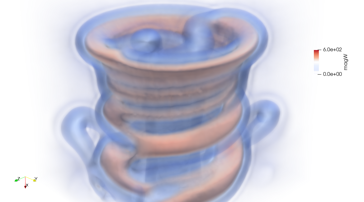

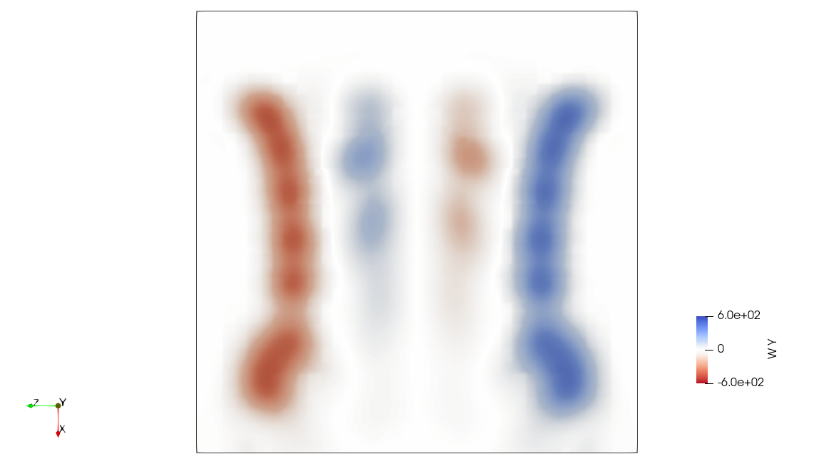
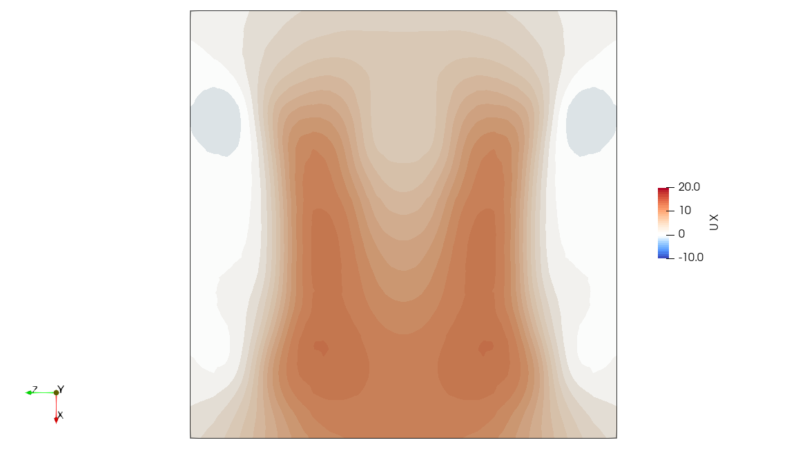
Mid-High Fidelity



High Fidelity