Heaving Wing
In this example we extend the simple wing case to create a case of interactional aerodynamics. We will place a straight wing flying in front of the original swept-back wing. The front wing will be moving in a heaving motion, shedding a wake that impinges on the back wing causing an unsteady loading.
This simulation exemplify the following features:
- Defining a
uns.VLMVehiclewith multiple surfaces, one of them declared as a tilting surface - Defining the control inputs for a tilting system in
uns.KinematicManeuver(in this case, tilting the surface over time in a heaving motion)
#=##############################################################################
# DESCRIPTION
    Swept-back wing flying in the wake of a tandem wing in heaving motion.

# AUTHORSHIP
  * Author          : Eduardo J. Alvarez (edoalvarez.com)
  * Email           : Edo.AlvarezR@gmail.com
  * Created         : Mar 2023
  * Last updated    : Mar 2023
  * License         : MIT
=###############################################################################

import FLOWUnsteady as uns
import FLOWVLM as vlm

run_name        = "heavingwing-example"    # Name of this simulation

save_path       = run_name                  # Where to save this simulation
paraview        = true                      # Whether to visualize with Paraview


# ----------------- GEOMETRY PARAMETERS ----------------------------------------
# Back wing description
b_back          = 2.489                     # (m) span length
ar_back         = 5.0                       # Aspect ratio b/c_tip
tr_back         = 1.0                       # Taper ratio c_tip/c_root
twist_root_back = 0.0                       # (deg) twist at root
twist_tip_back  = 0.0                       # (deg) twist at tip
lambda_back     = 45.0                      # (deg) sweep
gamma_back      = 0.0                       # (deg) dihedral

# Front wing description
b_front         = 0.75*b_back
ar_front        = 5.0
tr_front        = 1.0
twist_root_front= 5.0
twist_tip_front = 0.0
lambda_front    = 0.0
gamma_front     = 0.0

dx              = 0.75*b_back               # (m) spacing between back and front wings

# Discretization
n_back          = 50                        # Number of spanwise elements per side
r_back          = 2.0                       # Geometric expansion of elements
central_back    = false                     # Whether expansion is central

n_front         = 40
r_front         = 10.0
central_front   = false

# ----------------- SIMULATION PARAMETERS --------------------------------------
# Vehicle motion
magVvehicle     = 49.7                      # (m/s) vehicle velocity
AOA             = 4.2                       # (deg) angle of attack of back wing
frequency       = 25.0                      # (Hz) oscillation frequency in heaving motion
amplitude       = 5.0                       # (deg) AOA amplitude in heaving motion

# Freestream
magVinf         = 1e-8                      # (m/s) freestream velocity
rho             = 0.93                      # (kg/m^3) air density
qinf            = 0.5*rho*magVvehicle^2     # (Pa) static pressure (reference)

Vinf(X, t)      = t==0 ? magVvehicle*[1,0,0] : magVinf*[1,0,0] # Freestream function

# NOTE: In this simulation we will have the vehicle (the two wings) move while
#       the freestream is zero. However, a zero freestream can cause some
#       numerical instabilities in the solvers. To avoid instabilities, it is
#       recommended giving a full freestream velocity (or the velocity of the
#       vehicle) in the first time step `t=0`, and a negligible small velocity
#       at any other time, as shown above in the definition of `Vinf(X ,t)`.

magVref         = magVvehicle               # (m/s) reference velocity (for calculation
                                            # purposes since freestream is zero)

# ----------------- SOLVER PARAMETERS ------------------------------------------
# Time parameters
wakelength      = 4.0*b_back                # (m) length of wake to be resolved
ttot            = wakelength/magVref        # (s) total simulation time
nsteps          = 200                       # Number of time steps

# VLM and VPM parameters
p_per_step      = 2                         # Number of particle sheds per time step

sigma_vlm_solver= -1                        # VLM-on-VLM smoothing radius (deactivated with <0)
sigma_vlm_surf  = 0.05*b_back               # VLM-on-VPM smoothing radius
lambda_vpm      = 2.0                       # VPM core overlap
                                            # VPM smoothing radius
sigma_vpm_overwrite = lambda_vpm * magVref * (ttot/nsteps)/p_per_step

shed_starting   = true                      # Whether to shed starting vortex
vlm_rlx         = 0.7                       # VLM relaxation


# ----------------- 1) VEHICLE DEFINITION --------------------------------------
println("Generating geometry...")

# Generate back wing
backwing = vlm.simpleWing(b_back, ar_back, tr_back, twist_root_back,
                            lambda_back, gamma_back; twist_tip=twist_tip_back,
                            n=n_back, r=r_back, central=central_back);

# Pitch back wing to its angle of attack
O = [0.0, 0.0, 0.0]                                 # New position
Oaxis = uns.gt.rotation_matrix2(0.0, -AOA, 0.0)     # New orientation
vlm.setcoordsystem(backwing, O, Oaxis)

# Generate front wing
frontwing = vlm.simpleWing(b_front, ar_front, tr_front, twist_root_front,
                            lambda_front, gamma_front; twist_tip=twist_tip_front,
                            n=n_front, r=r_front, central=central_front);

# Move wing to the front
O = [-dx, 0.0, 0.0]                                 # New position
Oaxis = uns.gt.rotation_matrix2(0.0, 0.0, 0.0)      # New orientation
vlm.setcoordsystem(frontwing, O, Oaxis)


println("Generating vehicle...")

# Places the front wing into its own system that will be heaving
heavingsystem = vlm.WingSystem()            # Tilting system
vlm.addwing(heavingsystem, "FrontWing", frontwing)

# Generate vehicle
system = vlm.WingSystem()                   # System of all FLOWVLM objects
vlm.addwing(system, "BackWing", backwing)
vlm.addwing(system, "Heaving", heavingsystem)

tilting_systems = (heavingsystem, );        # Tilting systems

vlm_system = system;                        # System solved through VLM solver
wake_system = system;                       # System that will shed a VPM wake

vehicle = uns.VLMVehicle(   system;
                            tilting_systems=tilting_systems,
                            vlm_system=vlm_system,
                            wake_system=wake_system
                         );

# NOTE: Through the `tilting_systems` keyword argument to `uns.VLMVehicle` we
#       have declared that the front wing will be tilting throughout the
#       simulation, acting as a control surface. We will later declare the
#       control inputs to this tilting surface when we define the
#       `uns.KinematicManeuver`


# ------------- 2) MANEUVER DEFINITION -----------------------------------------

# Non-dimensional translational velocity of vehicle over time
Vvehicle(t) = [-1, 0, 0]        # <---- Vehicle is traveling in the -x direction

# Angle of the vehicle over time
anglevehicle(t) = zeros(3)

# Control inputs
angle_frontwing(t) = [0, amplitude*sin(2*pi*frequency * t*ttot), 0]  # Tilt angle of front wing

angle = (angle_frontwing, )                 # Angle of each tilting system
RPM = ()                                    # RPM of each rotor system (none)

maneuver = uns.KinematicManeuver(angle, RPM, Vvehicle, anglevehicle)

# NOTE: `FLOWUnsteady.KinematicManeuver` defines a maneuver with prescribed
#       kinematics. `Vvehicle` defines the velocity of the vehicle (a vector)
#       over time. `anglevehicle` defines the attitude of the vehicle over time.
#       `angle` defines the tilting angle of each tilting system over time.
#       `RPM` defines the RPM of each rotor system over time.
#       Each of these functions receives a nondimensional time `t`, which is the
#       simulation time normalized by the total time `ttot`, from 0 to
#       1, beginning to end of simulation. They all return a nondimensional
#       output that is then scaled by either a reference velocity (`Vref`) or
#       a reference RPM (`RPMref`). Defining the kinematics and controls of the
#       maneuver in this way allows the user to have more control over how fast
#       to perform the maneuver, since the total time, reference velocity and
#       RPM are then defined in the simulation parameters shown below.
At this point we can verify that we have correctly defined the control inputs of the maneuver calling FLOWUnsteady.plot_maneuver as follows:
uns.plot_maneuver(maneuver)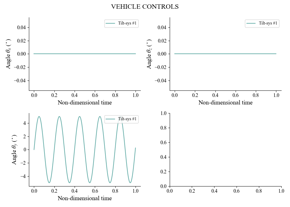
Here we confirm that the angle of the tilting surface along the $y$-axis of the vehicle (pitch) will change sinusoidally with amplitude $5^\circ$, as expected. This function also plots the kinematics of the vehicle, which in this case are rather uneventful (straight line).
Now we continue defining the simulation:
# ------------- 3) SIMULATION DEFINITION ---------------------------------------

Vref = magVvehicle                          # Reference velocity to scale maneuver by
RPMref = 0.0                                # Reference RPM to scale maneuver by
Vinit = Vref*Vvehicle(0)                    # Initial vehicle velocity
Winit = pi/180*(anglevehicle(1e-6) - anglevehicle(0))/(1e-6*ttot)  # Initial angular velocity

                                            # Maximum number of particles
max_particles = (nsteps+1)*(vlm.get_m(vehicle.vlm_system)*(p_per_step+1) + p_per_step)

simulation = uns.Simulation(vehicle, maneuver, Vref, RPMref, ttot;
                                                    Vinit=Vinit, Winit=Winit);


# ------------- 4) MONITORS DEFINITIONS ----------------------------------------

figs, figaxs = [], []                       # Figures generated by monitors

# Generate function that computes aerodynamic forces
calc_aerodynamicforce_fun = uns.generate_calc_aerodynamicforce(;
                                    add_parasiticdrag=true,
                                    add_skinfriction=true,
                                    airfoilpolar="xf-rae101-il-1000000.csv"
                                    )

L_dir(t) = [0, 0, 1]                        # Direction of lift
D_dir(t) = [1, 0, 0]                        # Direction of drag

# Generate back wing monitor
monitor_backwing = uns.generate_monitor_wing(backwing, Vinf, b_back, ar_back,
                                            rho, qinf, nsteps;
                                            calc_aerodynamicforce_fun=calc_aerodynamicforce_fun,
                                            L_dir=L_dir,
                                            D_dir=D_dir,
                                            out_figs=figs,
                                            out_figaxs=figaxs,
                                            save_path=save_path,
                                            run_name=run_name*"-backwing",
                                            title_lbl="Back Wing",
                                            figname="back-wing monitor",
                                            )

# Generate front wing monitor
monitor_frontwing = uns.generate_monitor_wing(frontwing, Vinf, b_front, ar_front,
                                            rho, qinf, nsteps;
                                            calc_aerodynamicforce_fun=calc_aerodynamicforce_fun,
                                            L_dir=L_dir,
                                            D_dir=D_dir,
                                            out_figs=figs,
                                            out_figaxs=figaxs,
                                            save_path=save_path,
                                            run_name=run_name*"-frontwing",
                                            title_lbl="Front Wing",
                                            figname="front-wing monitor",
                                            )

monitors = uns.concatenate(monitor_backwing, monitor_frontwing)


# ------------- 5) RUN SIMULATION ----------------------------------------------
println("Running simulation...")

uns.run_simulation(simulation, nsteps;
                    # ----- SIMULATION OPTIONS -------------
                    Vinf=Vinf,
                    rho=rho,
                    # ----- SOLVERS OPTIONS ----------------
                    p_per_step=p_per_step,
                    max_particles=max_particles,
                    sigma_vlm_solver=sigma_vlm_solver,
                    sigma_vlm_surf=sigma_vlm_surf,
                    sigma_rotor_surf=sigma_vlm_surf,
                    sigma_vpm_overwrite=sigma_vpm_overwrite,
                    vlm_rlx=vlm_rlx,
                    shed_starting=shed_starting,
                    extra_runtime_function=monitors,
                    # ----- OUTPUT OPTIONS ------------------
                    save_path=save_path,
                    run_name=run_name,
                    );


# ----------------- 6) VISUALIZATION -------------------------------------------
if paraview
    println("Calling Paraview...")

    # Files to open in Paraview
    files = joinpath(save_path, run_name*"_BackWing_vlm...vtk;")
    files *= run_name*"_Heaving_FrontWing_vlm...vtk;"
    files *= run_name*"_pfield...xmf;"

    # Call Paraview
    run(`paraview --data=$(files)`)

end
Reduce resolution (`n` and `nsteps`) to speed up simulation without loss of accuracy.
As the simulation runs, you will see the monitors (shown below) plotting the lift and drag coefficients over time along with the loading distribution.
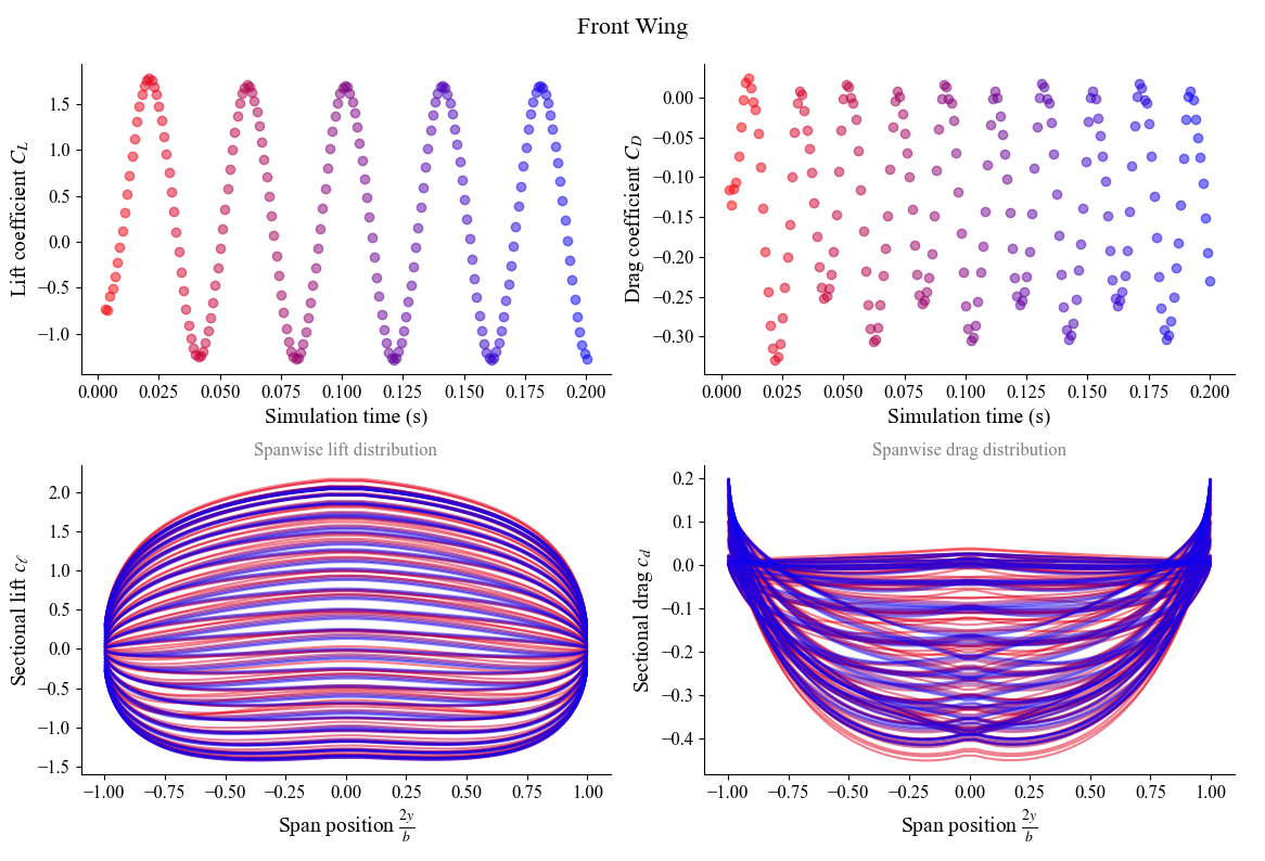
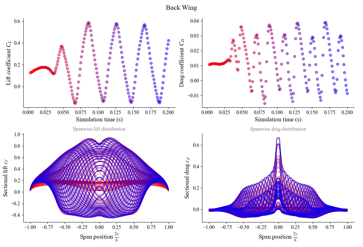
(red = beginning, blue = end)
In these monitors, we clearly see the fluctuation of $C_L$ and $C_D$ over time due to the heaving motion (front wing) and the wake impingement (back wing). The plots of loading distribution seem very convoluted since the loading fluctuates over time, and all the time steps are super imposed in the monitor.
To more clearly see what the loading distribution is doing, it is insightful to plot the loading as an animation as shown below.
Check the full example under examples/heavingwing/ to see how to postprocess the simulation and generate this animation.
FLOWUnsteady also provides a quasi-steady solver for low-fidelity simulations that replaces the particle field with rigid semi-infinite wakes. The quasi-steady solver is invoked by simply changing the line that defines the vehicle from
vehicle = uns.VLMVehicle(...)to
vehicle = uns.QVLMVehicle(...)(yes, it is only one character of a difference)
Use the keyword argument save_horseshoes = false in uns.run_simulation to visualize the semi-infinite rigid wake. The quasi-steady simulation looks like this: