Prop-on-Wing Interactions

In this example we use the actuator surface model (ASM) to more accurately predict the effects of props blowing on a wing. This case simulates the PROWIM experiment in Leo Veldhuis' dissertation (2005), and reproduces the validation study published in Alvarez & Ning (2023).

In this example you can vary the fidelity of the simulation setting the following parameters:

• $^\star$RK3: vpm_integration = vpm.rungekutta3
• $^\dag$None: vpm_SFS = vpm.SFS_none
• $^\ddag$Dynamic: vpm_SFS = vpm.SFS_Cd_twolevel_nobackscatter

(Low fidelity settings may be inadequate for accurately capturing prop-on-wing interactions, but mid-low or higher should do well)

As a reference, high-fidelity looks like this (except that the video shows a tip-mounted configuration with ailerons):

#=##############################################################################
# DESCRIPTION
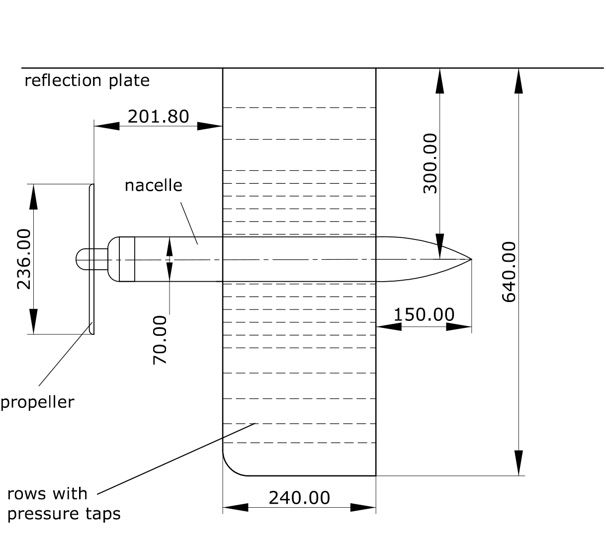
    Validation of prop-on-wing interactions with twin props mounted mid span
    blowing on a wing. This case simulates the PROWIM experiment in Leo
    Veldhuis' dissertation (2005), “Propeller Wing Aerodynamic Interference.”

    In this simulation we use the actuator surface model for the wing in order
    to accurately capture prop-on-wing interactional effects. The rotors still
    use the actuator line model.

    The high-fidelity settings replicate the results presented in Alvarez &
    Ning (2023), "Meshless Large-Eddy Simulation of Propeller–Wing Interactions
    with Reformulated Vortex Particle Method," Sec. IV.B, also available in
    Alvarez (2022), "Reformulated Vortex Particle Method and Meshless Large Eddy
    Simulation of Multirotor Aircraft," Sec. 8.4.

# ABOUT
  * Author          : Eduardo J. Alvarez (edoalvarez.com)
  * Email           : Edo.AlvarezR@gmail.com
  * Created         : January 2024
  * Last updated    : January 2024
  * License         : MIT
=###############################################################################


import FLOWUnsteady as uns
import FLOWUnsteady: vlm, vpm

run_name        = "prowim"                  # Name of this simulation
save_path       = run_name*"-example2"       # Where to save this simulation
prompt          = true                      # Whether to prompt the user
paraview        = true                      # Whether to visualize with Paraview

add_wing        = true                      # Whether to add wing to simulation
add_rotors      = true                      # Whether to add rotors to simulation

# ----------------- GEOMETRY PARAMETERS ----------------------------------------
# Wing geometry
b               = 2*0.64                    # (m) span length
ar              = 5.33                      # Aspect ratio b/c_tip
tr              = 1.0                       # Taper ratio c_tip/c_root
twist_root      = 0.0                       # (deg) twist at root
twist_tip       = 0.0                       # (deg) twist at tip
lambda          = 0.0                       # (deg) sweep
gamma           = 0.0                       # (deg) dihedral
thickness_w     = 0.15                      # Thickness t/c of wing airfoil

# Rotor geometry
rotor_file      = "beaver.csv"              # Rotor geometry
data_path       = uns.def_data_path         # Path to rotor database
read_polar      = vlm.ap.read_polar2        # What polar reader to use
pitch           = 2.5                       # (deg) collective pitch of blades
xfoil           = false                     # Whether to run XFOIL
ncrit           = 6                         # Turbulence criterion for XFOIL

# Read radius of this rotor and number of blades
R, B            = uns.read_rotor(rotor_file; data_path=data_path)[[1,3]]

# Vehicle assembly
AOAwing         = 0.0                       # (deg) wing angle of attack
spanpos         = [-0.46875, 0.46875]       # Semi-span position of each rotor, 2*y/b
xpos            = [-0.8417, -0.8417]        # x-position of rotors relative to LE, x/c
zpos            = [0.0, 0.0]                # z-position of rotors relative to LE, z/c
CWs             = [false, true]             # Rotation direction of each rotor: outboard up
# CWs             = [true, false]           # Rotation direction of each rotor: inboard up
nrotors         = length(spanpos)           # Number of rotors

# Discretization
n_wing          = 50                        # Number of spanwise elements per side
r_wing          = 2.0                       # Geometric expansion of elements
# n_rotor         = 20                        # Number of blade elements per blade
n_rotor         = 12
r_rotor         = 1/10                      # Geometric expansion of elements

# Check that we declared all the inputs that we need for each rotor
@assert nrotors==length(spanpos)==length(xpos)==length(zpos)==length(CWs) ""*
    "Invalid rotor inputs! Check that spanpos, xpos, zpos, and CWs have the same length"

# ----------------- SIMULATION PARAMETERS --------------------------------------
# Freestream
magVinf         = 49.5                      # (m/s) freestream velocity
AOA             = 4.0                       # (deg) vehicle angle of attack
rho             = 1.225                     # (kg/m^3) air density
mu              = 1.79e-5                   # (kg/ms) air dynamic viscosity
speedofsound    = 342.35                    # (m/s) speed of sound
qinf            = 0.5*rho*magVinf^2         # (Pa) reference static pressure
Vinf(X, t)      = magVinf*[cosd(AOA), 0, sind(AOA)]  # Freestream function

# Rotor operation
J               = 0.85                      # Advance ratio Vinf/(nD)
RPM             = 60*magVinf/(J*2*R)        # RPM

# Reference non-dimensional parameters
Rec             = rho * magVinf * (b/ar) / mu       # Chord-based wing Reynolds number
ReD             = 2*pi*RPM/60*R * rho/mu * 2*R      # Diameter-based rotor Reynolds number
Mtip            = 2*pi*RPM/60 * R / speedofsound    # Tip Mach number

println("""
    Vinf:   $(round(magVinf, digits=1)) m/s
    RPM:    $(RPM)
    Mtip:   $(round(Mtip, digits=3))
    ReD:    $(round(ReD, digits=0))
    Rec:    $(round(Rec, digits=0))
""")


# NOTE: Modify the variable `AOA` in order to change the angle of attack.
#       `AOAwing` will only change the angle of attack of the wing (while
#       leaving the propellers unaffected), while `AOA` changes the angle of
#       attack of the freestream (affecting both wing and props).

# ----------------- SOLVER PARAMETERS ------------------------------------------

# Aerodynamic solver
VehicleType     = uns.UVLMVehicle           # Unsteady solver
# VehicleType     = uns.QVLMVehicle         # Quasi-steady solver
const_solution  = VehicleType==uns.QVLMVehicle  # Whether to assume that the
                                                # solution is constant or not
# Time parameters
nrevs           = 8                         # Number of revolutions in simulation
nsteps_per_rev  = 36                        # Time steps per revolution
nsteps          = const_solution ? 2 : nrevs*nsteps_per_rev # Number of time steps
ttot            = nsteps/nsteps_per_rev / (RPM/60)       # (s) total simulation time

# VPM particle shedding
# p_per_step      = 5                         # Sheds per time step
p_per_step      = 2
shed_starting   = false                     # Whether to shed starting vortex (NOTE: starting vortex might make simulation unstable with AOA>8)
shed_unsteady   = false                     # Whether to shed vorticity from unsteady loading
unsteady_shedcrit = 0.001                   # Shed unsteady loading whenever circulation
                                            #  fluctuates by more than this ratio
treat_wake      = true                      # Treat wake to avoid instabilities
max_particles   = 1                         # Maximum number of particles
max_particles   += add_rotors * (nrotors*((2*n_rotor+1)*B)*nsteps*p_per_step)
max_particles   += add_wing * (nsteps+1)*(2*n_wing*(p_per_step+1) + p_per_step)

# Regularization
sigma_vlm_surf  = b/200                     # VLM-on-VPM smoothing radius (σLBV of wing)
sigma_rotor_surf= R/80                      # Rotor-on-VPM smoothing radius (σ of rotor)
lambda_vpm      = 2.125                     # VPM core overlap
                                            # VPM smoothing radius (σ of wakes)
sigma_vpm_overwrite = lambda_vpm * 2*pi*R/(nsteps_per_rev*p_per_step)

# Rotor solver
vlm_rlx         = 0.3                       # VLM relaxation <-- this also applied to rotors
hubtiploss_correction = ( (0.75, 10, 0.5, 0.05), (1, 1, 1, 1.0) ) # Hub/tip correction
# VPM solver
# vpm_integration = vpm.rungekutta3           # VPM temporal integration scheme
vpm_integration = vpm.euler

vpm_viscous     = vpm.Inviscid()            # VPM viscous diffusion scheme
                                            # Uncomment this to make it viscous
# vpm_viscous   = vpm.CoreSpreading(-1, -1, vpm.zeta_fmm; beta=100.0, itmax=20, tol=1e-1)

vpm_SFS       = vpm.SFS_none              # VPM LES subfilter-scale model
# vpm_SFS         = vpm.DynamicSFS(vpm.Estr_fmm, vpm.pseudo3level_positive;
                                  # alpha=0.999, maxC=1.0,
                                  # clippings=[vpm.clipping_backscatter])

# NOTE: By default we make this simulation inviscid since at such high Reynolds
#       number the viscous effects in the wake are actually negligible.
#       Notice that while viscous diffusion is negligible, turbulent diffusion
#       is important and non-negigible, so we have activated the subfilter-scale
#       (SFS) model.

if VehicleType == uns.QVLMVehicle
    # Mute warnings regarding potential colinear vortex filaments. This is
    # needed since the quasi-steady solver will probe induced velocities at the
    # lifting line of the blade
    uns.vlm.VLMSolver._mute_warning(true)
end

println("""
    Resolving wake for $(round(ttot*magVinf/b, digits=1)) span distances
""")





# ----------------- ACTUATOR SURFACE MODEL PARAMETERS (WING) -------------------

# ---------- Vortex sheet parameters ---------------
vlm_vortexsheet = true                      # Spread wing circulation as a vortex sheet (activates the ASM)
vlm_vortexsheet_overlap = 2.125/10          # Particle overlap in vortex sheet
vlm_vortexsheet_distribution = uns.g_pressure   # Distribution of the vortex sheet

vlm_vortexsheet_sigma_tbv = thickness_w*(b/ar) / 128 # Smoothing radius of trailing bound vorticity, σTBV for VLM-on-VPM

vlm_vortexsheet_maxstaticparticle = 10^6    # Particles to preallocate for vortex sheet

if add_wing && vlm_vortexsheet
    max_particles += vlm_vortexsheet_maxstaticparticle
end


# ---------- Force calculation parameters ----------
KJforce_type                = "regular"     # KJ force evaluated at middle of bound vortices
# KJforce_type              = "averaged"    # KJ force evaluated at average vortex sheet
# KJforce_type              = "weighted"    # KJ force evaluated at strength-weighted vortex sheet

include_trailingboundvortex = false         # Include trailing bound vortices in force calculations

include_freevortices        = false         # Include free vortices in force calculation
include_freevortices_TBVs   = false         # Include trailing bound vortex in free-vortex force

include_unsteadyforce       = true          # Include unsteady force
add_unsteadyforce           = false         # Whether to add the unsteady force to Ftot or to simply output it

include_parasiticdrag       = true          # Include parasitic-drag force
add_skinfriction            = true          # If false, the parasitic drag is purely form, meaning no skin friction
calc_cd_from_cl             = true          # Whether to calculate cd from cl or effective AOA
# calc_cd_from_cl             = false

# NOTE: We use a polar at a low Reynolds number (100k as opposed to 600k from
#       the experiment) as this particular polar better resembles the drag of
#       the tripped airfoil used in the experiment
wing_polar_file             = "xf-n64015a-il-100000-n5.csv"    # Airfoil polar for parasitic drag (from airfoiltools.com)


if include_freevortices && Threads.nthreads()==1
    @warn("Free-vortex force calculation requested, but Julia was initiated"*
          " with only one CPU thread. This will be extremely slow!"*
          " Initate Julia with `-t num` where num is the number of cores"*
          " availabe to speed up the computation.")
end





# ----------------- WAKE TREATMENT ---------------------------------------------

wake_treatments = []

# Remove particles by particle strength: remove particles neglibly weak, remove
# particles potentially blown up
rmv_strngth = 2.0 * magVinf*(b/ar)/2 * magVinf*ttot/nsteps/p_per_step  # Reference strength (maxCL=2.0)
minmaxGamma = rmv_strngth*[0.0001, 10.0]    # Strength bounds (removes particles outside of these bounds)
wake_treatment_strength = uns.remove_particles_strength( minmaxGamma[1]^2, minmaxGamma[2]^2; every_nsteps=1)

if treat_wake
    push!(wake_treatments, wake_treatment_strength)
end





# ----------------- 1) VEHICLE DEFINITION --------------------------------------

# -------- Generate components
println("Generating geometry...")

# Generate wing
wing = vlm.simpleWing(b, ar, tr, twist_root, lambda, gamma;
                                    twist_tip=twist_tip, n=n_wing, r=r_wing);

# Pitch wing to its angle of attack
O = [0.0, 0.0, 0.0]                                 # New position
Oaxis = uns.gt.rotation_matrix2(0, -AOAwing, 0)     # New orientation
vlm.setcoordsystem(wing, O, Oaxis)

# Generate rotors
rotors = vlm.Rotor[]
for ri in 1:nrotors

    # Generate rotor
    rotor = uns.generate_rotor(rotor_file;
                                pitch=pitch,
                                n=n_rotor, CW=CWs[ri], blade_r=r_rotor,
                                altReD=[RPM, J, mu/rho],
                                xfoil=xfoil,
                                ncrit=ncrit,
                                data_path=data_path,
                                read_polar=read_polar,
                                verbose=true,
                                verbose_xfoil=false,
                                plot_disc=false
                                );

    # Simulate only one rotor if the wing is not in the simulation
    if !add_wing
        push!(rotors, rotor)
        break
    end

    # Determine position along wing LE
    y = spanpos[ri]*b/2
    x = abs(y)*tand(lambda) + xpos[ri]*b/ar
    z = abs(y)*tand(gamma) + zpos[ri]*b/ar

    # Account for angle of attack of wing
    nrm = sqrt(x^2 + z^2)
    x = (x==0 ? 1 : sign(x))*nrm*cosd(AOAwing)
    z = -(z==0 ? 1 : sign(z))*nrm*sind(AOAwing)

    # Translate rotor to its position along wing
    O_r = [x, y, z]                                     # New position
    Oaxis_r = uns.gt.rotation_matrix2(0, 0, 0)          # New orientation
    vlm.setcoordsystem(rotor, O_r, Oaxis_r; user=true)

    push!(rotors, rotor)
end


# -------- Generate vehicle
println("Generating vehicle...")

# System of all FLOWVLM objects
system = vlm.WingSystem()

if add_wing
    vlm.addwing(system, "Wing", wing)
end

if add_rotors
    for (ri, rotor) in enumerate(rotors)
        vlm.addwing(system, "Rotor$(ri)", rotor)
    end
end

# System solved through VLM solver
vlm_system = vlm.WingSystem()
add_wing ? vlm.addwing(vlm_system, "Wing", wing) : nothing

# Systems of rotors
rotor_systems = add_rotors ? (rotors, ) : NTuple{0, Array{vlm.Rotor, 1}}()

# System that will shed a VPM wake
wake_system = vlm.WingSystem()              # System that will shed a VPM wake
add_wing ? vlm.addwing(wake_system, "Wing", wing) : nothing
                                            # NOTE: Do NOT include rotor when using the quasi-steady solver
if VehicleType != uns.QVLMVehicle && add_rotors
    for (ri, rotor) in enumerate(rotors)
        vlm.addwing(wake_system, "Rotor$(ri)", rotor)
    end
end

# Pitch vehicle to its angle of attack (0 in this case since we have tilted the freestream instead)
O = [0.0, 0.0, 0.0]                                 # New position
Oaxis = uns.gt.rotation_matrix2(0, 0, 0)            # New orientation
vlm.setcoordsystem(system, O, Oaxis)

vehicle = VehicleType(   system;
                            vlm_system=vlm_system,
                            rotor_systems=rotor_systems,
                            wake_system=wake_system
                         );






# ------------- 2) MANEUVER DEFINITION -----------------------------------------
# Non-dimensional translational velocity of vehicle over time
Vvehicle(t) = [-1, 0, 0]        # <---- Vehicle is traveling in the -x direction

# Angle of the vehicle over time
anglevehicle(t) = zeros(3)

# RPM control input over time (RPM over `RPMref`)
RPMcontrol(t) = 1.0

angles = ()                                 # Angle of each tilting system (none)
RPMs = add_rotors ? (RPMcontrol, ) : ()     # RPM of each rotor system

maneuver = uns.KinematicManeuver(angles, RPMs, Vvehicle, anglevehicle)






# ------------- 3) SIMULATION DEFINITION ---------------------------------------

Vref = 0.0                                  # Reference velocity to scale maneuver by
RPMref = RPM                                # Reference RPM to scale maneuver by
Vinit = Vref*Vvehicle(0)                    # Initial vehicle velocity
Winit = pi/180*(anglevehicle(1e-6) - anglevehicle(0))/(1e-6*ttot)  # Initial angular velocity

simulation = uns.Simulation(vehicle, maneuver, Vref, RPMref, ttot;
                                                    Vinit=Vinit, Winit=Winit);





# ------------- *) AERODYNAMIC FORCES ------------------------------------------
# Here we define the different components of aerodynamic of force that we desire
# to capture with the wing using the actuator surface model

forces = []

# Calculate Kutta-Joukowski force
kuttajoukowski = uns.generate_aerodynamicforce_kuttajoukowski(KJforce_type,
                                sigma_vlm_surf, sigma_rotor_surf,
                                vlm_vortexsheet, vlm_vortexsheet_overlap,
                                vlm_vortexsheet_distribution,
                                vlm_vortexsheet_sigma_tbv;
                                vehicle=vehicle)
push!(forces, kuttajoukowski)

# Free-vortex force
if include_freevortices
    freevortices = uns.generate_calc_aerodynamicforce_freevortices(
                                            vlm_vortexsheet_maxstaticparticle,
                                            sigma_vlm_surf,
                                            vlm_vortexsheet,
                                            vlm_vortexsheet_overlap,
                                            vlm_vortexsheet_distribution,
                                            vlm_vortexsheet_sigma_tbv;
                                            Ffv=uns.Ffv_direct,
                                            include_TBVs=include_freevortices_TBVs
                                            )
    push!(forces, freevortices)
end

# Force due to unsteady circulation
if include_unsteadyforce
    unsteady(args...; optargs...) = uns.calc_aerodynamicforce_unsteady(args...;
                                      add_to_Ftot=add_unsteadyforce, optargs...)

    push!(forces, unsteady)
end

# Parasatic-drag force (form drag and skin friction)
if include_parasiticdrag
    parasiticdrag = uns.generate_aerodynamicforce_parasiticdrag(
                            wing_polar_file;
                            read_path=joinpath(data_path, "airfoils"),
                            calc_cd_from_cl=calc_cd_from_cl,
                            add_skinfriction=add_skinfriction,
                            Mach=speedofsound!=nothing ? magVinf/speedofsound : nothing
                            )

    push!(forces, parasiticdrag)
end


# Stitch all the forces into one function
function calc_aerodynamicforce_fun(vlm_system, args...; per_unit_span=false, optargs...)

    # Delete any previous force field
    fieldname = per_unit_span ? "ftot" : "Ftot"
    if fieldname in keys(vlm_system.sol)
        pop!(vlm_system.sol, fieldname)
    end

    Ftot = nothing

    for (fi, force) in enumerate(forces)
        Ftot = force(vlm_system, args...; per_unit_span=per_unit_span, optargs...)
    end

    return Ftot
end






# ------------- 4) MONITORS DEFINITIONS ----------------------------------------

# Generate wing monitor
L_dir = [-sind(AOA), 0, cosd(AOA)]          # Direction of lift
D_dir = [ cosd(AOA), 0, sind(AOA)]          # Direction of drag

monitor_wing = uns.generate_monitor_wing(wing, Vinf, b, ar,
                                            rho, qinf, nsteps;
                                            calc_aerodynamicforce_fun=calc_aerodynamicforce_fun,
                                            include_trailingboundvortex=include_trailingboundvortex,
                                            L_dir=L_dir,
                                            D_dir=D_dir,
                                            save_path=save_path,
                                            run_name=run_name*"-wing",
                                            figname="wing monitor",
                                            )

# Generate rotors monitor
monitor_rotors = uns.generate_monitor_rotors(rotors, J, rho, RPM, nsteps;
                                            t_scale=RPM/60,        # Scaling factor for time in plots
                                            t_lbl="Revolutions",   # Label for time axis
                                            save_path=save_path,
                                            run_name=run_name*"-rotors",
                                            figname="rotors monitor",
                                            )

# Generate monitor of flow enstrophy (indicates numerical stability)
monitor_enstrophy = uns.generate_monitor_enstrophy(;
                                            save_path=save_path,
                                            run_name=run_name,
                                            figname="enstrophy monitor"
                                            )

# Generate monitor of SFS model coefficient Cd
monitor_Cd = uns.generate_monitor_Cd(;      save_path=save_path,
                                            run_name=run_name,
                                            figname="Cd monitor"
                                            )


# Concatenate monitors
all_monitors = [monitor_enstrophy, monitor_Cd]

add_wing ? push!(all_monitors, monitor_wing) : nothing
add_rotors ? push!(all_monitors, monitor_rotors) : nothing

monitors = uns.concatenate(all_monitors...)

# Concatenate user-defined runtime function
extra_runtime_function = uns.concatenate(monitors, wake_treatments...)



# ------------- 5) RUN SIMULATION ----------------------------------------------
println("Running simulation...")


# Run simulation
uns.run_simulation(simulation, nsteps;

                    # ----- SIMULATION OPTIONS -------------
                    Vinf=Vinf,
                    rho=rho, mu=mu, sound_spd=speedofsound,

                    # ----- SOLVERS OPTIONS ----------------
                    vpm_integration=vpm_integration,
                    vpm_viscous=vpm_viscous,
                    vpm_SFS=vpm_SFS,

                    p_per_step=p_per_step,
                    max_particles=max_particles,

                    sigma_vpm_overwrite=sigma_vpm_overwrite,
                    sigma_rotor_surf=sigma_rotor_surf,
                    sigma_vlm_surf=sigma_vlm_surf,

                    vlm_rlx=vlm_rlx,
                    vlm_vortexsheet=vlm_vortexsheet,
                    vlm_vortexsheet_overlap=vlm_vortexsheet_overlap,
                    vlm_vortexsheet_distribution=vlm_vortexsheet_distribution,
                    vlm_vortexsheet_sigma_tbv=vlm_vortexsheet_sigma_tbv,
                    max_static_particles=vlm_vortexsheet_maxstaticparticle,

                    hubtiploss_correction=hubtiploss_correction,

                    shed_starting=shed_starting,
                    shed_unsteady=shed_unsteady,
                    unsteady_shedcrit=unsteady_shedcrit,

                    extra_runtime_function=extra_runtime_function,

                    # ----- OUTPUT OPTIONS ------------------
                    save_path=save_path,
                    run_name=run_name,
                    prompt=prompt,
                    save_wopwopin=false,  # <--- Generates input files for PSU-WOPWOP noise analysis if true

                    );






# ----------------- 6) VISUALIZATION -------------------------------------------
if paraview
    println("Calling Paraview...")

    # Files to open in Paraview
    files = joinpath(save_path, run_name*"_pfield...xmf;")

    if add_rotors
        for ri in 1:nrotors
            for bi in 1:B
                global files *= run_name*"_Rotor$(ri)_Blade$(bi)_loft...vtk;"
            end
        end
    end

    if add_wing
        files *= run_name*"_Wing_vlm...vtk;"
    end

    # Call Paraview
    run(`paraview --data=$(files)`)

end

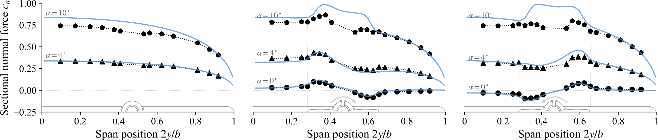
Mid-High Fidelity




High Fidelity

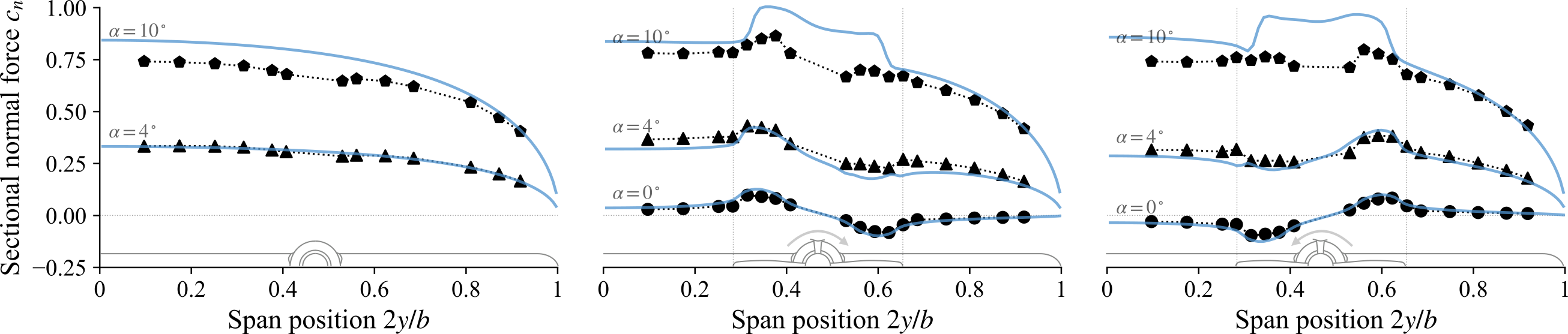
The favorable comparison with the experiment at $\alpha=0^\circ$ and $4^\circ$ confirms that ASM accurately predicts prop-on-wing interactions up to a moderate angle of attack. At $\alpha=10^\circ$ we suspect that the wing is mildly stalled in the experiment, leading to a larger discrepancy (further discussed in Alvarez' Dissertation^[1] and Alvarez & Ning, 2023^[2]).