Tethered Wing
In this example we extend the simple wing case to fly a circular path. This simulates a kite tethered to the ground with a crosswind that causes it to fly in circles. The kite effectively acts as a turbine extracting energy from the wind to sustain flight, which is the basis for the field of airborne wind energy.
This simulation exemplify the following features:
- Translating and re-orienting the initial position of the vehicle using
FLOWVLM.setcoordsystem - Defining a
uns.KinematicManeuverobject that prescribes the kinematics of a circular path - Customizing the wing monitor (
uns.generate_monitor_wing) to compute and plot forces decomposed in arbitrary directions (in this case, following the orientation of the vehicle along the circular path) - Monitoring the vehicle state variables with
uns.generate_monitor_statevariables
#=##############################################################################
# DESCRIPTION
    Kite flying in a circular path with crosswind while tethered to the ground.
    The kite is the same 45° swept-back wing from the previous example.

# AUTHORSHIP
  * Author          : Eduardo J. Alvarez (edoalvarez.com)
  * Email           : Edo.AlvarezR@gmail.com
  * Created         : Feb 2023
  * Last updated    : Feb 2023
  * License         : MIT
=###############################################################################

import FLOWUnsteady as uns
import FLOWVLM as vlm

run_name        = "tetheredwing-example"    # Name of this simulation

save_path       = run_name                  # Where to save this simulation
paraview        = true                      # Whether to visualize with Paraview


# ----------------- GEOMETRY PARAMETERS ----------------------------------------
# Wing description
b               = 2.489                     # (m) span length
ar              = 5.0                       # Aspect ratio b/c_tip
tr              = 1.0                       # Taper ratio c_tip/c_root
twist_root      = 0.0                       # (deg) twist at root
twist_tip       = 0.0                       # (deg) twist at tip
lambda          = 45.0                      # (deg) sweep
gamma           = 0.0                       # (deg) dihedral

# Discretization
n               = 50                        # Number of spanwise elements per side
r               = 10.0                      # Geometric expansion of elements
central         = false                     # Whether expansion is central

# ----------------- SIMULATION PARAMETERS --------------------------------------
# Freestream
magVinf         = 5.0                       # (m/s) freestream velocity
magVeff         = 49.7                      # (m/s) vehicle effective velocity
AOAeff          = 4.2                       # (deg) vehicle effective AOA
rho             = 0.93                      # (kg/m^3) air density
qinf            = 0.5*rho*magVeff^2         # (Pa) static pressure

Vinf(X, t)      = magVinf*[1, 0, 0]         # Freestream function

# Circular path
R               = 3.0*b                     # (m) radius of circular path
magVvehicle     = sqrt(magVeff^2 - magVinf^2) # (m/s) vehicle velocity
omega           = magVvehicle/R             # (rad/s) angular velocity
alpha           = AOAeff - atand(magVinf, magVvehicle) # (deg) vehicle pitch angle

# ----------------- SOLVER PARAMETERS ------------------------------------------
# Time parameters
nrevs           = 2.50                      # Revolutions to resolve
nsteps_per_rev  = 144                       # Number of time steps per revolution

ttot            = nrevs / (omega/(2*pi))    # (s) total simulation time
nsteps          = ceil(Int, nrevs * nsteps_per_rev) # Number of time steps

# VLM and VPM parameters
p_per_step      = 4                         # Number of particle sheds per time step

sigma_vlm_solver= -1                        # VLM-on-VLM smoothing radius (deactivated with <0)
sigma_vlm_surf  = 0.05*b                    # VLM-on-VPM smoothing radius
lambda_vpm      = 2.125                     # VPM core overlap
                                            # VPM smoothing radius
sigma_vpm_overwrite = lambda_vpm * magVeff * (ttot/nsteps)/p_per_step

shed_starting   = true                      # Whether to shed starting vortex
vlm_rlx         = 0.7                       # VLM relaxation

# NOTE: In some cases the starting vortex can cause numerical instabilities at
#       the beginning of the simulation. If so, consider omitting shedding of
#       the starting vortex with `shed_starting=false`, or relax the VLM solver
#       with `0.2 < vlm_rlx < 0.9`


# ----------------- 1) VEHICLE DEFINITION --------------------------------------
println("Generating geometry...")

# Generate wing
wing = vlm.simpleWing(b, ar, tr, twist_root, lambda, gamma;
                        twist_tip=twist_tip, n=n, r=r, central=central);

# Rotate wing to pitch
O = [0.0, 0.0, 0.0]                                 # New position
Oaxis = uns.gt.rotation_matrix2(0.0, -alpha, 0.0)   # New orientation
vlm.setcoordsystem(wing, O, Oaxis)


println("Generating vehicle...")

# Generate vehicle
system = vlm.WingSystem()                   # System of all FLOWVLM objects
vlm.addwing(system, "Wing", wing)

vlm_system = system;                        # System solved through VLM solver
wake_system = system;                       # System that will shed a VPM wake

vehicle = uns.VLMVehicle(   system;
                            vlm_system=vlm_system,
                            wake_system=wake_system
                         );

 # Rotate vehicle to be perpendicular to crosswind
 # and translate it to start at (x, y, z) = (0, R, 0)
 O = [0, R, 0]                                      # New position
 Oaxis = uns.gt.rotation_matrix2(0.0, -90, 0.0)     # New orientation

 vlm.setcoordsystem(system, O, Oaxis)


# ------------- 2) MANEUVER DEFINITION -----------------------------------------

# Translational velocity of vehicle over time
function Vvehicle(t)

    # NOTE: This function receives a non-dimensional time `t` (with t=0 being
    #       the start of simulation and t=1 the end), and returns a
    #       non-dimensional velocity vector. This vector will later be scaled
    #       by `Vref`.

    Vx = 0
    Vy = -sin(2*pi*nrevs*t)
    Vz = cos(2*pi*nrevs*t)

    return [0, Vy, Vz]
end

# Angle of the vehicle over time
function anglevehicle(t)

    # NOTE: This function receives the non-dimensional time `t` and returns the
    #       attitude of the vehicle (a vector with inclination angles with
    #       respect to each axis of the global coordinate system)

    return [0, 0, 360*nrevs*t]
end

angle = ()                                  # Angle of each tilting system (none)
RPM = ()                                    # RPM of each rotor system (none)

maneuver = uns.KinematicManeuver(angle, RPM, Vvehicle, anglevehicle)

# NOTE: `FLOWUnsteady.KinematicManeuver` defines a maneuver with prescribed
#       kinematics. `Vvehicle` defines the velocity of the vehicle (a vector)
#       over time. `anglevehicle` defines the attitude of the vehicle over time.
#       `angle` defines the tilting angle of each tilting system over time (none
#       in this case). `RPM` defines the RPM of each rotor system over time
#       (none in this case).
#       Each of these functions receives a nondimensional time `t`, which is the
#       simulation time normalized by the total time `ttot`, from 0 to
#       1, beginning to end of simulation. They all return a nondimensional
#       output that is then scaled by either a reference velocity (`Vref`) or
#       a reference RPM (`RPMref`). Defining the kinematics and controls of the
#       maneuver in this way allows the user to have more control over how fast
#       to perform the maneuver, since the total time, reference velocity and
#       RPM are then defined in the simulation parameters shown below.


# ------------- 3) SIMULATION DEFINITION ---------------------------------------

Vref = magVvehicle                          # Reference velocity to scale maneuver by
RPMref = 0.0                                # Reference RPM to scale maneuver by
Vinit = Vref*Vvehicle(0)                    # Initial vehicle velocity
Winit = pi/180*(anglevehicle(1e-6) - anglevehicle(0))/(1e-6*ttot)  # Initial angular velocity

                                            # Maximum number of particles
max_particles = (nsteps+1)*(vlm.get_m(vehicle.vlm_system)*(p_per_step+1) + p_per_step)

simulation = uns.Simulation(vehicle, maneuver, Vref, RPMref, ttot;
                                                    Vinit=Vinit, Winit=Winit);


# ------------- 4) MONITORS DEFINITIONS ----------------------------------------

figs, figaxs = [], []                       # Figures generated by monitors
import FLOWUnsteady: @L_str                 # Macro for writing LaTeX labels

# Generate function that computes aerodynamic forces
calc_aerodynamicforce_fun = uns.generate_calc_aerodynamicforce(;
                                    add_parasiticdrag=true,
                                    add_skinfriction=true,
                                    airfoilpolar="xf-rae101-il-1000000.csv"
                                    )

# Time-varying directions used to decompose the aerodynamic force
N_dir(t) = [1, 0, 0]                        # Direction of normal force
T_dir(t) = [0, sin(omega*t), -cos(omega*t)] # Direction of tangent force
S_dir(t) = uns.cross(N_dir(t), T_dir(t))    # Spanwise direction

X_offset(t) = system.O                      # Reference wing origin (for calculating spanwise position)
S_proj(t)   = S_dir(t)                      # Reference span direction (for calculating spanwise position)

# Generate wing monitor
monitor_wing = uns.generate_monitor_wing(wing, Vinf, b, ar,
                                            rho, qinf, nsteps;
                                            calc_aerodynamicforce_fun=calc_aerodynamicforce_fun,
                                            L_dir=N_dir,
                                            D_dir=T_dir,
                                            X_offset=X_offset,
                                            S_proj=S_proj,
                                            CL_lbl=L"Normal force $C_n$",
                                            CD_lbl=L"Tangent force $C_t$",
                                            cl_lbl=L"Sectional normal force $c_n$",
                                            cd_lbl=L"Sectional tangent force $c_t$",
                                            cl_ttl="Normal force distribution",
                                            cd_ttl="Tangent force distribution",
                                            out_figs=figs,
                                            out_figaxs=figaxs,
                                            save_path=save_path,
                                            run_name=run_name,
                                            figname="wing monitor",
                                            );

# Generate monitor of state variables
monitor_states = uns.generate_monitor_statevariables(; save_path=save_path,
                                                       run_name=run_name,
                                                       out_figs=figs,
                                                       out_figaxs=figaxs,
                                                       nsteps_savefig=10)

monitors = uns.concatenate(monitor_wing, monitor_states)


# ------------- 5) RUN SIMULATION ----------------------------------------------
println("Running simulation...")

uns.run_simulation(simulation, nsteps;
                    # ----- SIMULATION OPTIONS -------------
                    Vinf=Vinf,
                    rho=rho,
                    # ----- SOLVERS OPTIONS ----------------
                    p_per_step=p_per_step,
                    max_particles=max_particles,
                    sigma_vlm_solver=sigma_vlm_solver,
                    sigma_vlm_surf=sigma_vlm_surf,
                    sigma_rotor_surf=sigma_vlm_surf,
                    sigma_vpm_overwrite=sigma_vpm_overwrite,
                    vlm_rlx=vlm_rlx,
                    shed_starting=shed_starting,
                    extra_runtime_function=monitors,
                    # ----- OUTPUT OPTIONS ------------------
                    save_path=save_path,
                    run_name=run_name,
                    );


# ----------------- 6) VISUALIZATION -------------------------------------------
if paraview
    println("Calling Paraview...")

    # Files to open in Paraview
    files = joinpath(save_path, run_name*"_Wing_vlm...vtk")
    files *= ";"*run_name*"_pfield...xmf;"

    # Call Paraview
    run(`paraview --data=$(files)`)

end
Reduce resolution (n and steps) to speed up simulation without loss of accuracy.
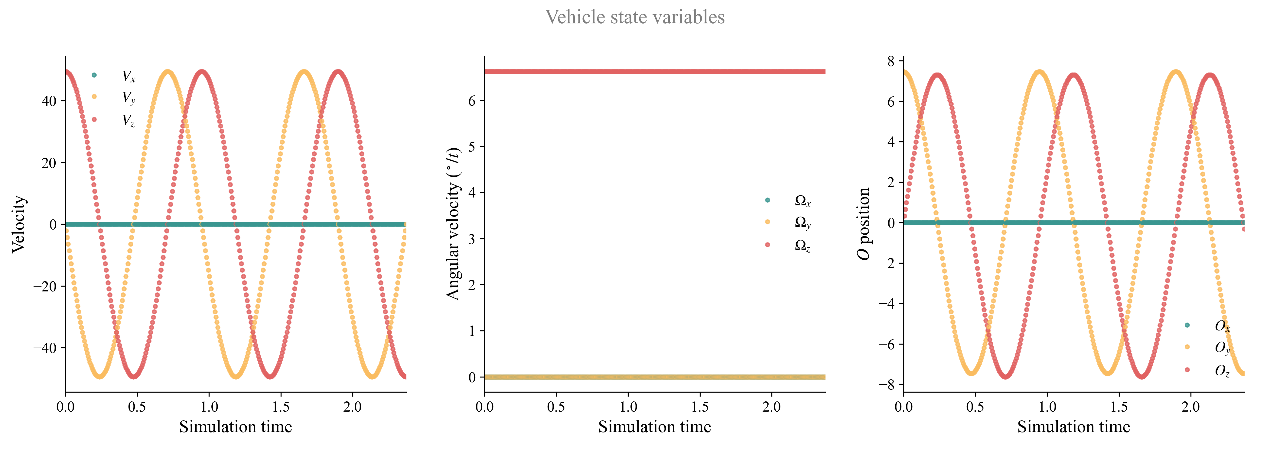
As the simulation runs, you will see the monitor shown below plotting the state variables of the vehicle. The components of both velocity and position follow a sinusoidal function, which is consistent with the circular path, while the angular velocity is constant.
The force monitor (shown below) plots the force components that are normal and tangential to the plane of rotation. Notice that the tangential force is negative, which is equivalent to having a negative drag, meaning that the vehicle is actually being propelled by the crosswind. Also notice that the forces are perturbed every time it completes a revolution. This is due to encountering the starting point of the wake that is slowly traveling downstream. It takes a couple revolutions for the forces to converge once the wake has been fully deployed.
(red = beginning, blue = end)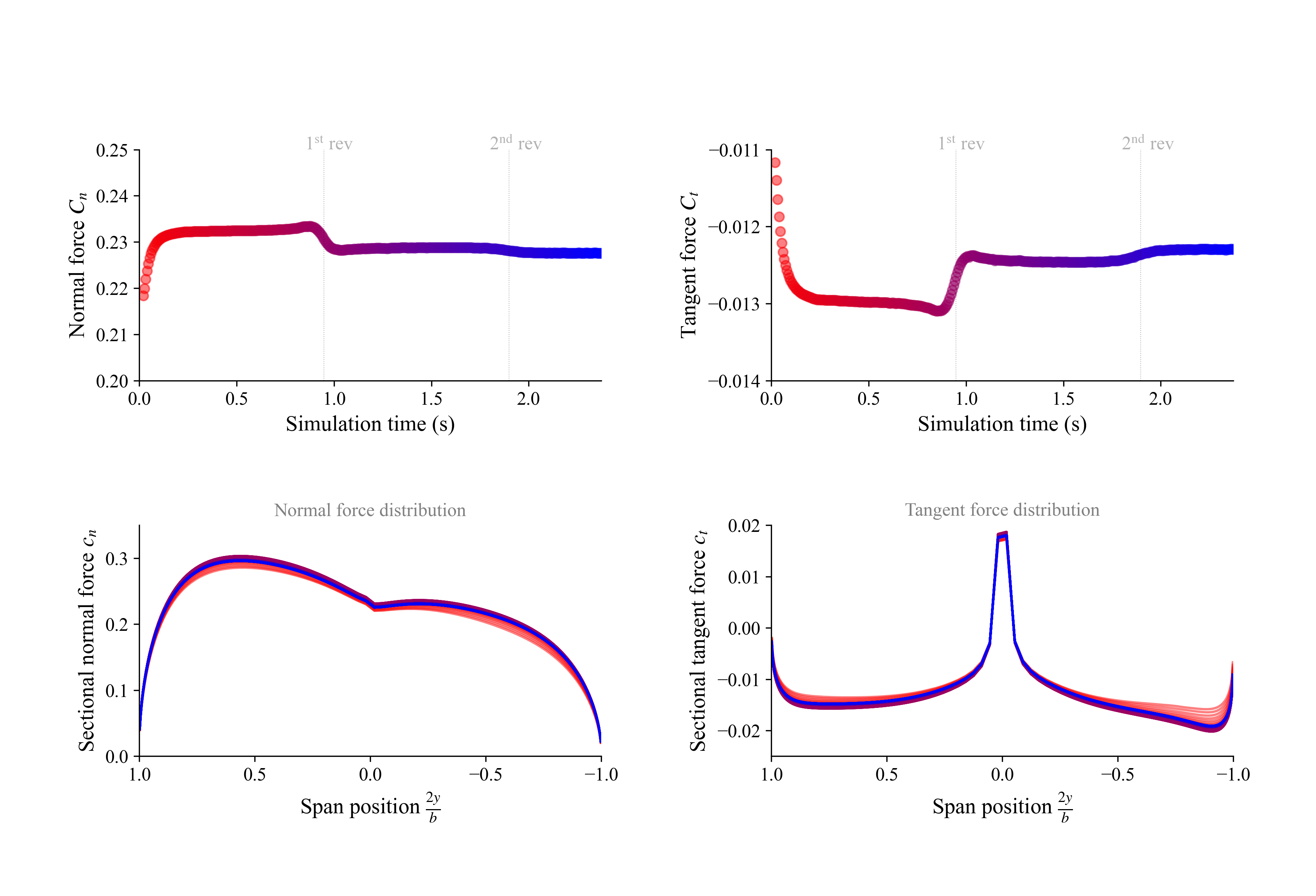
For unknown reasons, the simulation oftentimes halts in between time steps while plotting the monitors. This slows down the overall simulation time, sometimes taking up to 2x longer. If you are not particularly interested in the plots of the monitors, you can disable the plots passing the keyword disp_plot=false to each monitor generator.
The .pvsm file visualizing the simulation as shown at the top of this page is available here: LINK (right click → save as...).
To open in ParaView: File → Load State → (select .pvsm file) then select "Search files under specified directory" and point it to the folder where the simulation was saved.