Polynomial Chaos for Wind Farm Power Prediction
28 May 2019, Andrew Ning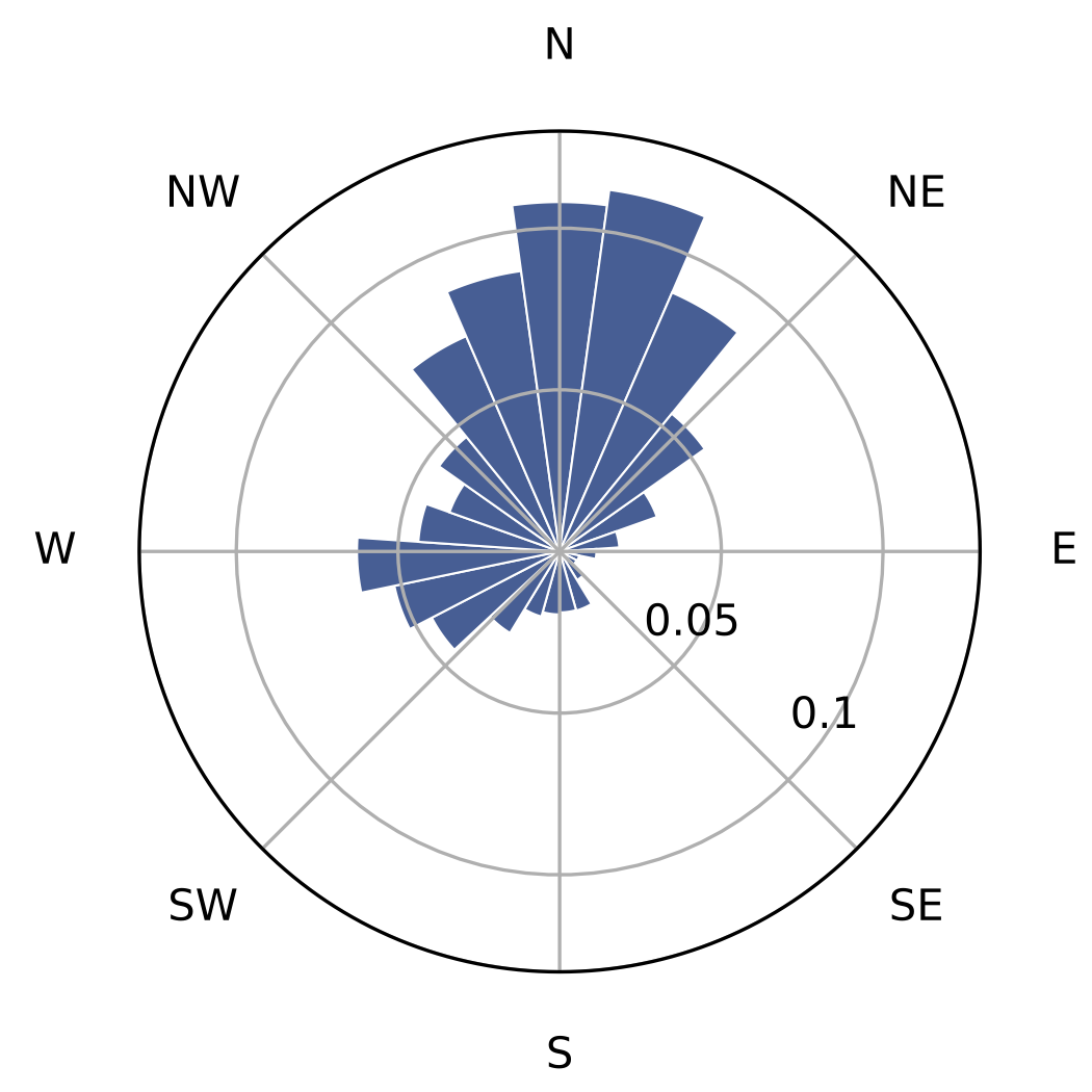
In a wind farm, it is important to understand how both the wind speed and wind direction varies. The variability in wind direction is captured in what is called a wind rose (see above). The longer bars in the wind rose indicate directions from which wind is more likely to come from. The power produced by the wind farm can change dramatically as the wind direction changes. This variation in power is often reduced to a single number—the expected value of power (an average). In the wind energy field, a common metric of interest is the annual energy production (AEP), which is the expected value of power (multiplied by time in a year and availability).
The wind rose is really a continuous distribution, but we often discretize it into bins like shown above. This discretization provides a convenient way to compute average power production. This is done by dividing the uncertain variable (wind direction in this example) into discrete bins, multiplying the power for each direction by its probability, then summing up over all bins. This approach is the familiar rectangle rule. It’s a simple approach and is almost always the approach used in wind farm analysis.
In a collaboration between our lab and the Aerospace Design Laboratory at Stanford we’ve been exploring an alternative approach based on polynomial chaos. Polynomial chaos is not a new method. It is widely known and used in applications of uncertainty quantification, but has not yet been applied to wind farm analysis. The main idea is that rather than discretize into bins, we can use polynomials to approximate the continuous power response, allowing us to use fewer samples to approximate the AEP.
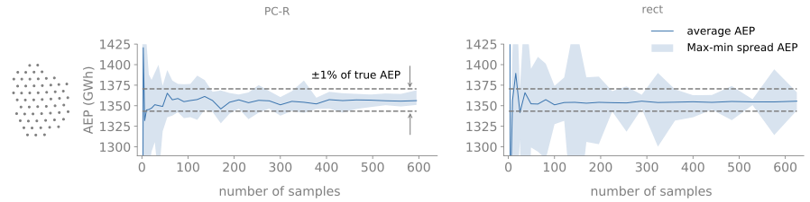
Santiago led a recent study where we explored using polynomial chaos, with uncertainty in both wind direction and wind speed, to predict AEP. We explored using both quadrature approaches and regression approaches and found the latter to be more effective. On average, polynomial chaos reduced the number of simulations required by a factor of 5 as compared to the rectangle rule. For example, the figure below shows how AEP varies with the number of samples with polynomial chaos based on regression to the left, and the rectangle rule to the right. We see that polynomial chaos converges with fewer samples and produces less variability in the AEP estimates from starting the quadrature at different points.
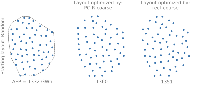
Additionally, we applied polynomial chaos to optimizing wind farm layouts. We found that using polynomial chaos with regression allowed for about 1/3 of the simulations required for the rectangle rule (while producing a slightly better AEP). One such case is shown below.
Further details are available in the open-access paper and data linked below.
- Padrón, A. S., Thomas, J., Stanley, A. P. J., Alonso, J. J., and Ning, A., “Polynomial Chaos to Efficiently Compute the Annual Energy Production in Wind Farm Layout Optimization,” Wind Energy Science, Vol. 4, pp. 211–231, May 2019. doi:10.5194/wes-4-211-2019
[BibTeX] [DOI] [PDF] [Code]
@article{Padron2019,
  author = {Padr\'{o}n, A. Santiago and Thomas, Jared and Stanley, Andrew P. J. and Alonso, Juan J. and Ning, Andrew},
  doi = {10.5194/wes-4-211-2019},
  journal = {Wind Energy Science},
  month = may,
  pages = {211-231},
  title = {Polynomial Chaos to Efficiently Compute the Annual Energy Production in Wind Farm Layout Optimization},
  volume = {4},
  year = {2019}
}