Using GXBeam with DifferentialEquations.jl
While the capabilities provided by GXBeam are probably sufficient for most users, advanced users may wish to make use of some of the features of the DifferentialEquations package. For this reason, we have created an interface in GXBeam to allow users to model the differential algebraic equations encountered in GXBeam using DifferentialEquations.
This guide is also available as a Jupyter notebook: diffeq.ipynb.
Interface Functions
The following constructors are available for modeling the differential algebraic equations from GXBeam in DifferentialEquations.
SciMLBase.ODEFunction — Method
SciMLBase.ODEFunction(system::AbstractSystem, assembly;
# general keyword arguments
prescribed_conditions=Dict{Int,PrescribedConditions{Float64}}(),
distributed_loads=Dict{Int,DistributedLoads{Float64}}(),
point_masses=Dict{Int,PointMass{Float64}}(),
linear_velocity=(@SVector zeros(3)),
angular_velocity=(@SVector zeros(3)),
gravity=(@SVector zeros(3)),
# control flag keyword arguments
structural_damping=true,
two_dimensional=false,
constant_mass_matrix=true,
sparse=false,
# sensitivity analysis keyword arguments
xpfunc = nothing,
pfunc = (p, t) -> (;),
p = nothing,
# additional keyword arguments (passed to ODEFunction constructor)
kwargs...)
Construct a ODEFunction for the system of nonlinear beams contained in assembly which may be used with the DifferentialEquations package.
General Keyword Arguments
prescribed_conditions = Dict{Int,PrescribedConditions{Float64}}(): A dictionary with keys corresponding to the points at which prescribed conditions are applied and values of typePrescribedConditionswhich describe the prescribed conditions at those points. If time varying, this input may be provided as a function of time.distributed_loads = Dict{Int,DistributedLoads{Float64}}(): A dictionary with keys corresponding to the elements to which distributed loads are applied and values of typeDistributedLoadswhich describe the distributed loads on those elements. If time varying, this input may be provided as a function of time.point_masses = Dict{Int,PointMass{Float64}}(): A dictionary with keys corresponding to the points to which point masses are attached and values of typePointMasswhich contain the properties of the attached point masses. If time varying, this input may be provided as a function of time.linear_velocity = zeros(3): Prescribed linear velocity of the body frame.angular_velocity = zeros(3): Prescribed angular velocity of the body frame.gravity = [0,0,0]: Gravity vector in the body frame. If time varying, this input may be provided as a function of time.
Control Flag Keyword Arguments
structural_damping = true: Flag indicating whether to enable structural dampingtwo_dimensional = false: Flag indicating whether to constrain results to the x-y planeconstant_mass_matrix = true: Flag indicating whether to use a constant mass matrix.sparse = false: Flag indicating whether to use a sparse jacobian.
Sensitivity Analysis Keyword Arguments
pfunc = (p, t) -> (;): Function which returns a named tuple with fields corresponding to updated versions of the argumentsassembly,prescribed_conditions,distributed_loads,point_masses,linear_velocity,angular_velocity, andgravity. Only fields contained in the resulting named tuple will be overwritten.p: Sensitivity parameters, as defined in conjunction with the keyword argumentpfunc. While not necessary, usingpfuncandpto define the arguments to this function allows automatic differentiation sensitivities to be computed more efficiently
Additional keyword arguments are passed on to the ODEFunction constructor.
SciMLBase.ODEProblem — Method
ODEProblem(system::GXBeam.AbstractSystem, assembly, tspan; kwargs...)Construct an ODEProblem corresponding to the system of nonlinear beams contained in assembly. This problem may be solved using the DifferentialEquations package
General Keyword Arguments
prescribed_conditions = Dict{Int,PrescribedConditions{Float64}}(): A dictionary with keys corresponding to the points at which prescribed conditions are applied and values of typePrescribedConditionswhich describe the prescribed conditions at those points. If time varying, this input may be provided as a function of time.distributed_loads = Dict{Int,DistributedLoads{Float64}}(): A dictionary with keys corresponding to the elements to which distributed loads are applied and values of typeDistributedLoadswhich describe the distributed loads on those elements. If time varying, this input may be provided as a function of time.point_masses = Dict{Int,PointMass{Float64}}(): A dictionary with keys corresponding to the points to which point masses are attached and values of typePointMasswhich contain the properties of the attached point masses. If time varying, this input may be provided as a function of time.linear_velocity = zeros(3): Prescribed linear velocity of the body frame. If time varying, this input may be provided as a function of time.angular_velocity = zeros(3): Prescribed angular velocity of the body frame. If time varying, this input may be provided as a function of time.gravity = [0,0,0]: Gravity vector in the body frame. If time varying, this input may be provided as a function of time.
Control Flag Keyword Arguments
initial_state = nothing: Object of typeAssemblyState, which defines the initial states and state rates corresponding to the analysis. By default, this input is calculated using eithersteady_state_analysisorinitial_condition_analysis.structural_damping = true: Flag indicating whether to enable structural dampingtwo_dimensional = false: Flag indicating whether to constrain results to the x-y planeconstant_mass_matrix = true: Flag indicating whether to use a constant mass matrix.sparse = false: Flag indicating whether to use a sparse jacobian.
Sensitivity Analysis Keyword Arguments
xpfunc = (x, p, t) -> (;): Similar topfunc, except that parameters can also be defined as a function of GXBeam's state variables. Using this function forces the system jacobian to be computed using automatic differentiation.pfunc = (p, t) -> (;): Function which returns a named tuple with fields corresponding to updated versions of the argumentsassembly,prescribed_conditions,distributed_loads,point_masses,linear_velocity,angular_velocity, andgravity. Only fields contained in the resulting named tuple will be overwritten.p: Sensitivity parameters, as defined in conjunction with the keyword argumentpfunc. While not necessary, usingpfuncandpto define the arguments to this function allows automatic differentiation sensitivities to be computed more efficiently
Additional keyword arguments are passed on to the ODEProblem constructor.
SciMLBase.DAEFunction — Method
DAEFunction(system::GXBeam.AbstractSystem, assembly; kwargs...)Construct a DAEFunction for the system of nonlinear beams contained in assembly which may be used with the DifferentialEquations package.
General Keyword Arguments
prescribed_conditions = Dict{Int,PrescribedConditions{Float64}}(): A dictionary with keys corresponding to the points at which prescribed conditions are applied and values of typePrescribedConditionswhich describe the prescribed conditions at those points. If time varying, this input may be provided as a function of time.distributed_loads = Dict{Int,DistributedLoads{Float64}}(): A dictionary with keys corresponding to the elements to which distributed loads are applied and values of typeDistributedLoadswhich describe the distributed loads on those elements. If time varying, this input may be provided as a function of time.point_masses = Dict{Int,PointMass{Float64}}(): A dictionary with keys corresponding to the points to which point masses are attached and values of typePointMasswhich contain the properties of the attached point masses. If time varying, this input may be provided as a function of time.linear_velocity = zeros(3): Prescribed linear velocity of the body frame.angular_velocity = zeros(3): Prescribed angular velocity of the body frame.gravity = [0,0,0]: Gravity vector in the body frame. If time varying, this input may be provided as a function of time.
Control Flag Keyword Arguments
structural_damping = true: Flag indicating whether to enable structural dampingtwo_dimensional = false: Flag indicating whether to constrain results to the x-y planeconstant_mass_matrix = true: Flag indicating whether to use a constant mass matrix.sparse = false: Flag indicating whether to use a sparse jacobian.
Sensitivity Analysis Keyword Arguments
xpfunc = (x, p, t) -> (;): Similar topfunc, except that parameters can also be defined as a function of GXBeam's state variables. Using this function forces the system jacobian to be computed using automatic differentiation.pfunc = (p, t) -> (;): Function which returns a named tuple with fields corresponding to updated versions of the argumentsassembly,prescribed_conditions,distributed_loads,point_masses,linear_velocity,angular_velocity, andgravity. Only fields contained in the resulting named tuple will be overwritten.p: Sensitivity parameters, as defined in conjunction with the keyword argumentpfunc. While not necessary, usingpfuncandpto define the arguments to this function allows automatic differentiation sensitivities to be computed more efficiently
Additional keyword arguments are passed on to the DAEFunction constructor.
SciMLBase.DAEProblem — Method
DAEProblem(system::GXBeam.AbstractSystem, assembly, tspan; kwargs...)Construct an DAEProblem corresponding to the system of nonlinear beams contained in assembly. This problem may be solved using the DifferentialEquations package
General Keyword Arguments
prescribed_conditions = Dict{Int,PrescribedConditions{Float64}}(): A dictionary with keys corresponding to the points at which prescribed conditions are applied and values of typePrescribedConditionswhich describe the prescribed conditions at those points. If time varying, this input may be provided as a function of time.distributed_loads = Dict{Int,DistributedLoads{Float64}}(): A dictionary with keys corresponding to the elements to which distributed loads are applied and values of typeDistributedLoadswhich describe the distributed loads on those elements. If time varying, this input may be provided as a function of time.point_masses = Dict{Int,PointMass{Float64}}(): A dictionary with keys corresponding to the points to which point masses are attached and values of typePointMasswhich contain the properties of the attached point masses. If time varying, this input may be provided as a function of time.linear_velocity = zeros(3): Prescribed linear velocity of the body frame. If time varying, this input may be provided as a function of time.angular_velocity = zeros(3): Prescribed angular velocity of the body frame. If time varying, this input may be provided as a function of time.gravity = [0,0,0]: Gravity vector in the body frame. If time varying, this input may be provided as a function of time.
Control Flag Keyword Arguments
initial_state = nothing: Object of typeAssemblyState, which defines the initial states and state rates corresponding to the analysis. By default, this input is calculated using eithersteady_state_analysisorinitial_condition_analysis.structural_damping = true: Flag indicating whether to enable structural dampingtwo_dimensional = false: Flag indicating whether to constrain results to the x-y planeconstant_mass_matrix = true: Flag indicating whether to use a constant mass matrix.sparse = false: Flag indicating whether to use a sparse jacobian.
Sensitivity Analysis Keyword Arguments
xpfunc = (x, p, t) -> (;): Similar topfunc, except that parameters can also be defined as a function of GXBeam's state variables. Using this function forces the system jacobian to be computed using automatic differentiation.pfunc = (p, t) -> (;): Function which returns a named tuple with fields corresponding to updated versions of the argumentsassembly,prescribed_conditions,distributed_loads,point_masses,linear_velocity,angular_velocity, andgravity. Only fields contained in the resulting named tuple will be overwritten.p: Sensitivity parameters, as defined in conjunction with the keyword argumentpfunc. While not necessary, usingpfuncandpto define the arguments to this function allows automatic differentiation sensitivities to be computed more efficiently
Additional keyword arguments are passed on to the DAEProblem constructor.
Example Usage
For this example we demonstrate how to solve the wind turbine Time-Domain Simulation of a Wind Turbine Blade problem using DifferentialEquations.
We start by setting up the problem as if we were solving the problem using GXBeam's internal solver.
using GXBeam, LinearAlgebra

L = 60 # m

# create points
nelem = 10
x = range(0, L, length=nelem+1)
y = zero(x)
z = zero(x)
points = [[x[i],y[i],z[i]] for i = 1:length(x)]

# index of endpoints of each beam element
start = 1:nelem
stop = 2:nelem+1

# stiffness matrix for each beam element
stiffness = fill(
    [2.389e9  1.524e6  6.734e6 -3.382e7 -2.627e7 -4.736e8
     1.524e6  4.334e8 -3.741e6 -2.935e5  1.527e7  3.835e5
     6.734e6 -3.741e6  2.743e7 -4.592e5 -6.869e5 -4.742e6
    -3.382e7 -2.935e5 -4.592e5  2.167e7 -6.279e5  1.430e6
    -2.627e7  1.527e7 -6.869e5 -6.279e5  1.970e7  1.209e7
    -4.736e8  3.835e5 -4.742e6  1.430e6  1.209e7  4.406e8],
    nelem)

# mass matrix for each beam element
mass = fill(
    [258.053      0.0        0.0      0.0      7.07839  -71.6871
       0.0      258.053      0.0     -7.07839  0.0        0.0
       0.0        0.0      258.053   71.6871   0.0        0.0
       0.0       -7.07839   71.6871  48.59     0.0        0.0
       7.07839    0.0        0.0      0.0      2.172      0.0
     -71.6871     0.0        0.0      0.0      0.0       46.418],
     nelem)

# create assembly of interconnected nonlinear beams
assembly = Assembly(points, start, stop; stiffness=stiffness, mass=mass)

# prescribed conditions
prescribed_conditions = (t) -> begin
    Dict(
        # fixed left side
        1 => PrescribedConditions(ux=0, uy=0, uz=0, theta_x=0, theta_y=0, theta_z=0),
        # force on right side
        nelem+1 => PrescribedConditions(Fz = 1e5*sin(20*t))
    )
end
At this point if we wanted to use GXBeam's internal solver, we would choose a time discretization and call the time_domain_analysis function.
# simulation time
t = 0:0.001:2.0

system, gxbeam_history, converged = time_domain_analysis(assembly, t;
    prescribed_conditions = prescribed_conditions,
    structural_damping = false)
To instead use the capabilities of the DifferentialEquations package, we first initialize our system using the initial_condition_analysis function and then construct and solve a DAEProblem.
using DifferentialEquations

# define simulation time
tspan = (0.0, 2.0)

# run initial condition analysis to get consistent set of initial conditions
dae_system, converged = initial_condition_analysis(assembly, tspan[1];
    prescribed_conditions = prescribed_conditions,
    structural_damping = false)

# construct an ODEProblem (with a constant mass matrix)
dae_prob = DAEProblem(dae_system, assembly, tspan;
    prescribed_conditions = prescribed_conditions,
    structural_damping = false)

# solve the problem
dae_sol = solve(dae_prob, DABDF2())
Alternatively, we can use a mass matrix formulation of our differential algebraic equations.
# run initial condition analysis to get consistent set of initial conditions
ode_system, converged = initial_condition_analysis(assembly, tspan[1];
    prescribed_conditions = prescribed_conditions,
    constant_mass_matrix = true,
    structural_damping = false)

# construct an ODEProblem (with a constant mass matrix)
ode_prob = ODEProblem(ode_system, assembly, tspan;
    prescribed_conditions = prescribed_conditions,
    constant_mass_matrix = true,
    structural_damping = false)

# solve the problem
ode_sol = solve(ode_prob, Rodas4())
We can then extract the outputs from the solution in a easy to understand format using the AssemblyState constructor.
ode_history = [AssemblyState(ode_sol[it], ode_system, assembly; prescribed_conditions)
    for it in eachindex(ode_sol)]

dae_history = [AssemblyState(dae_sol[it], dae_system, assembly; prescribed_conditions)
    for it in eachindex(dae_sol)]
Let's now compare the solutions from GXBeam's internal solver and the DifferentialEquations solvers.
using Plots
pyplot()


point = vcat(fill(nelem+1, 6), fill(1, 6))
field = [:u, :u, :u, :theta, :theta, :theta, :F, :F, :F, :M, :M, :M]
direction = [1, 2, 3, 1, 2, 3, 1, 2, 3, 1, 2, 3]
ylabel = ["\$u_x\$ (\$m\$)", "\$u_y\$ (\$m\$)", "\$u_z\$ (\$m\$)",
    "Rodriguez Parameter \$\\theta_x\$ (degree)",
    "Rodriguez Parameter \$\\theta_y\$ (degree)",
    "Rodriguez Parameter \$\\theta_z\$ (degree)",
    "\$F_x\$ (\$N\$)", "\$F_y\$ (\$N\$)", "\$F_z\$ (\$N\$)",
    "\$M_x\$ (\$Nm\$)", "\$M_y\$ (\$Nm\$)", "\$M_z\$ (\$N\$)"]

for i = 1:12
    plot(
        xlim = (0, 2.0),
        xticks = 0:0.5:2.0,
        xlabel = "Time (s)",
        ylabel = ylabel[i],
        grid = false,
        overwrite_figure=false
        )
    y_gxbeam = [getproperty(state.points[point[i]], field[i])[direction[i]]
        for state in gxbeam_history]

    y_ode = [getproperty(state.points[point[i]], field[i])[direction[i]]
        for state in ode_history]

    y_dae = [getproperty(state.points[point[i]], field[i])[direction[i]]
        for state in dae_history]

    if field[i] == :theta
        # convert to Rodriguez parameter
        @. y_gxbeam = 4*atan(y_gxbeam/4)
        @. y_ode = 4*atan(y_ode/4)
        @. y_dae = 4*atan(y_dae/4)
        # convert to degrees
        @. y_gxbeam = rad2deg(y_gxbeam)
        @. y_ode = rad2deg(y_ode)
        @. y_dae = rad2deg(y_dae)
    end

    if field[i] == :F || field[i] == :M
        y_gxbeam = -y_gxbeam
        y_ode = -y_ode
        y_dae = -y_dae
    end

    plot!(t, y_gxbeam, label="GXBeam")
    plot!(ode_sol.t, y_ode, label="ODEProblem")
    plot!(dae_sol.t, y_dae, label="DAEProblem")
    plot!(show=true)
end


As can be seen, the solutions provided by GXBeam and DifferentialEquations track closely with each other.
root_chord = 1.9000
tip_chord =  0.4540
airfoil = [ # MH-104
    1.00000000  0.00000000;
    0.99619582  0.00017047;
    0.98515158  0.00100213;
    0.96764209  0.00285474;
    0.94421447  0.00556001;
    0.91510964  0.00906779;
    0.88074158  0.01357364;
    0.84177999  0.01916802;
    0.79894110  0.02580144;
    0.75297076  0.03334313;
    0.70461763  0.04158593;
    0.65461515  0.05026338;
    0.60366461  0.05906756;
    0.55242353  0.06766426;
    0.50149950  0.07571157;
    0.45144530  0.08287416;
    0.40276150  0.08882939;
    0.35589801  0.09329359;
    0.31131449  0.09592864;
    0.26917194  0.09626763;
    0.22927064  0.09424396;
    0.19167283  0.09023579;
    0.15672257  0.08451656;
    0.12469599  0.07727756;
    0.09585870  0.06875796;
    0.07046974  0.05918984;
    0.04874337  0.04880096;
    0.03081405  0.03786904;
    0.01681379  0.02676332;
    0.00687971  0.01592385;
    0.00143518  0.00647946;
    0.00053606  0.00370956;
    0.00006572  0.00112514;
    0.00001249 -0.00046881;
    0.00023032 -0.00191488;
    0.00079945 -0.00329201;
    0.00170287 -0.00470585;
    0.00354717 -0.00688469;
    0.00592084 -0.00912202;
    0.01810144 -0.01720842;
    0.03471169 -0.02488211;
    0.05589286 -0.03226730;
    0.08132751 -0.03908459;
    0.11073805 -0.04503763;
    0.14391397 -0.04986836;
    0.18067874 -0.05338180;
    0.22089879 -0.05551392;
    0.26433734 -0.05636585;
    0.31062190 -0.05605816;
    0.35933893 -0.05472399;
    0.40999990 -0.05254383;
    0.46204424 -0.04969990;
    0.51483073 -0.04637175;
    0.56767889 -0.04264894;
    0.61998250 -0.03859653;
    0.67114514 -0.03433153;
    0.72054815 -0.02996944;
    0.76758733 -0.02560890;
    0.81168064 -0.02134397;
    0.85227225 -0.01726049;
    0.88883823 -0.01343567;
    0.92088961 -0.00993849;
    0.94797259 -0.00679919;
    0.96977487 -0.00402321;
    0.98607009 -0.00180118;
    0.99640466 -0.00044469;
    1.00000000  0.00000000;
]

sections = zeros(3, size(airfoil, 1), length(points))
for ip = 1:length(points)
    chord = root_chord * (1 - x[ip]/L) + tip_chord * x[ip]/L
    sections[1, :, ip] .= 0
    sections[2, :, ip] .= chord .* (airfoil[:,1] .- 0.5)
    sections[3, :, ip] .= chord .* airfoil[:,2]
end

mkpath("dynamic-wind-turbine")
write_vtk("dynamic-wind-turbine/dynamic-wind-turbine", assembly, gxbeam_history, t; sections = sections)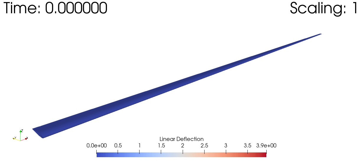
This page was generated using Literate.jl.