Variable Fidelity
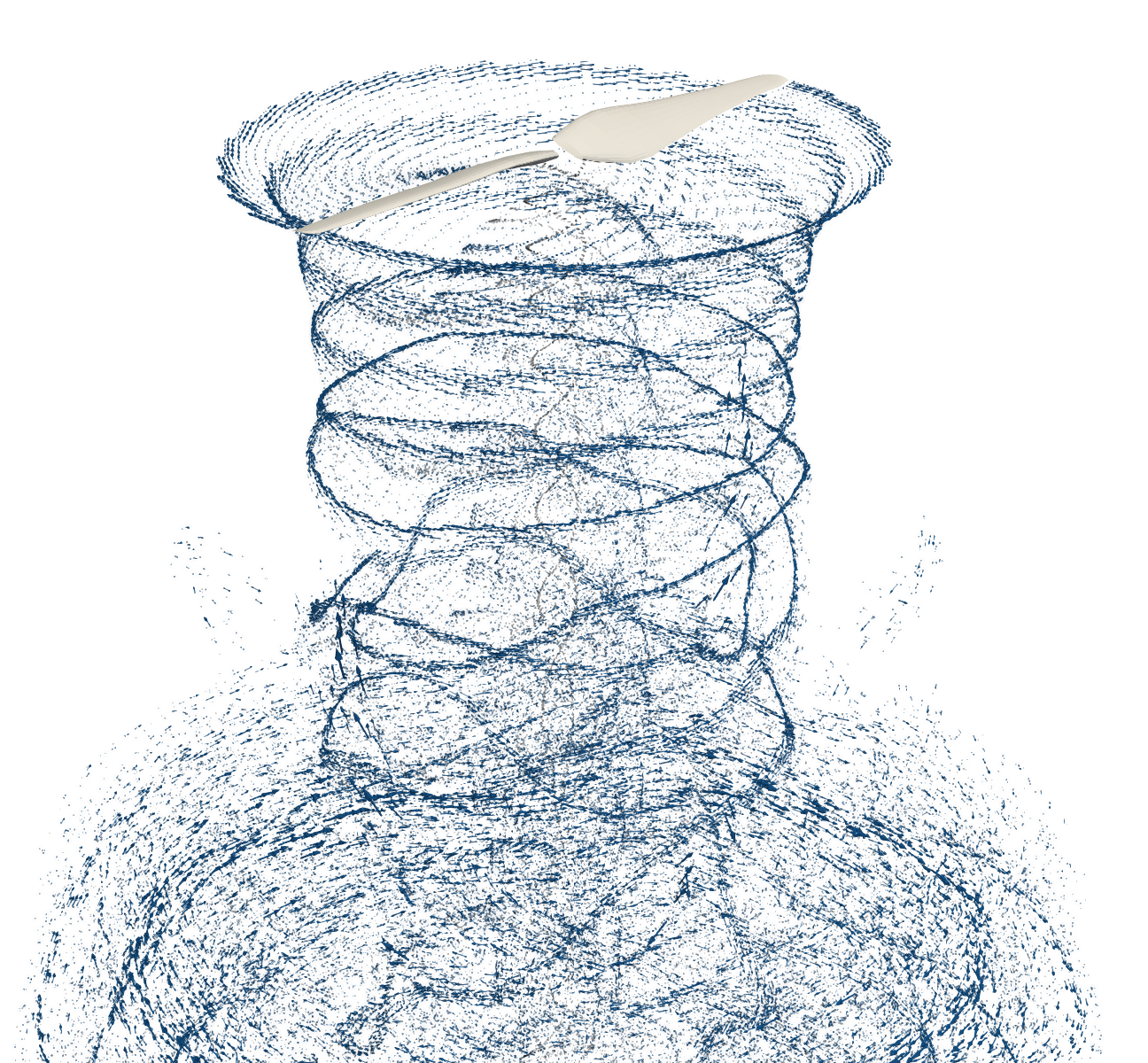
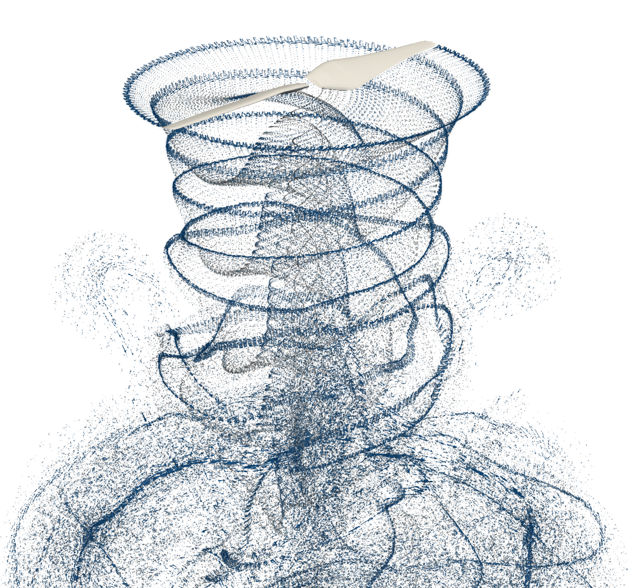
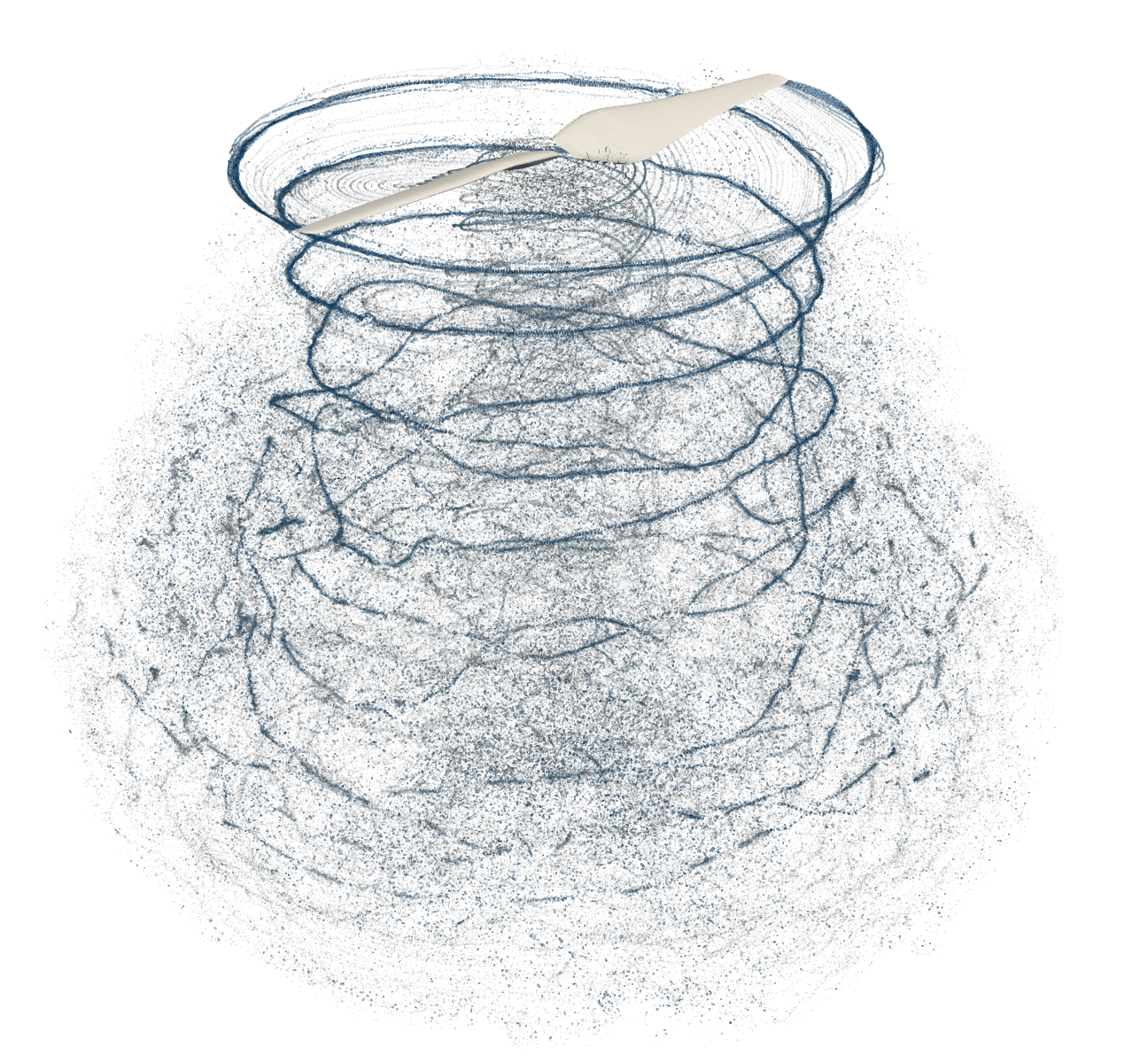
While propeller simulations tend to be numerically well behaved, a hover case can pose multiple numerical challenges. The rotation of blades in static air drives a strong axial flow that is solely caused by the shedding of tip vortices. This is challenging to simulate since, in the absence of a freestream, the wake quickly becomes fully turbulent and breaks down as tip vortices leapfrog and mix close to the rotor. Thus, a rotor in hover is a good engineering application to showcase the numerical stability and accuracy of FLOWUnsteady.
In this example we simulate a DJI rotor in hover, and we use this case to demonstrate some of the advanced features of FLOWUnsteady that make it robust and accurate in resolving turbulent mixing:
- Subfilter scale (SFS) model of turbulence related to vortex stretching
- How to monitor the dynamic SFS model coefficient with
uns.generate_monitor_Cd - How to monitor the global flow enstrophy with
uns.generate_monitor_enstrophyand track numerical stability - Defining a wake treatment procedure to suppress initial hub wake, avoiding hub fountain effects and accelerating convergence
- Defining hub and tip loss corrections
Also, in this example you can vary the fidelity of the simulation setting the following parameters:
| Parameter | Mid-low fidelity | Mid-high fidelity | High fidelity | Description |
|---|---|---|---|---|
n | 20 | 50 | 50 | Number of blade elements per blade |
nsteps_per_rev | 36 | 72 | 360 | Time steps per revolution |
p_per_step | 4 | 2 | 2 | Particle sheds per time step |
sigma_rotor_surf | R/10 | R/10 | R/80 | Rotor-on-VPM smoothing radius |
sigmafactor_vpmonvlm | 1.0 | 1.0 | 5.5 | Expand particles by this factor when calculating VPM-on-VLM/Rotor induced velocities |
shed_starting | false | false | true | Whether to shed starting vortex |
suppress_fountain | true | true | false | Whether to suppress hub fountain effect |
vpm_integration | vpm.euler | RK3$^\star$ | RK3$^\star$ | VPM time integration scheme |
vpm_SFS | None$^\dag$ | None$^\dag$ | Dynamic$^\ddag$ | VPM LES subfilter-scale model |
- $^\star$RK3:
vpm_integration = vpm.rungekutta3 - $^\dag$None:
vpm_SFS = vpm.SFS_none - $^\ddag$Dynamic:
vpm_SFS = vpm.SFS_Cd_twolevel_nobackscatter
70k particles ~7 mins. |
200k particles ~60 mins. |
1M particles ~30 hrs. |
#=##############################################################################
# DESCRIPTION
    Simulation of a DJI 9443 rotor in hover (two-bladed rotor, 9.4 inches
    diameter).

    This example replicates the experiment described in Zawodny & Boyd (2016),
    "Acoustic Characterization and Prediction of Representative,
    Small-scale Rotary-wing Unmanned Aircraft System Components."

# AUTHORSHIP
  * Author          : Eduardo J. Alvarez (edoalvarez.com)
  * Email           : Edo.AlvarezR@gmail.com
  * Created         : Mar 2023
  * Last updated    : Mar 2023
  * License         : MIT
=###############################################################################


import FLOWUnsteady as uns
import FLOWVLM as vlm
import FLOWVPM as vpm

run_name        = "rotorhover-example"      # Name of this simulation
save_path       = run_name                  # Where to save this simulation
paraview        = true                      # Whether to visualize with Paraview

# ----------------- GEOMETRY PARAMETERS ----------------------------------------

# Rotor geometry
rotor_file      = "DJI9443.csv"             # Rotor geometry
data_path       = uns.def_data_path         # Path to rotor database
pitch           = 0.0                       # (deg) collective pitch of blades
CW              = false                     # Clock-wise rotation
xfoil           = false                     # Whether to run XFOIL
read_polar      = vlm.ap.read_polar2        # What polar reader to use

# NOTE: If `xfoil=true`, XFOIL will be run to generate the airfoil polars used
#       by blade elements before starting the simulation. XFOIL is run
#       on the airfoil contours found in `rotor_file` at the corresponding
#       local Reynolds and Mach numbers along the blade.
#       Alternatively, the user can provide pre-computer airfoil polars using
#       `xfoil=false` and providing the polar files through `rotor_file`.
#       `read_polar` is the function that will be used to parse polar files. Use
#       `vlm.ap.read_polar` for files that are direct outputs of XFOIL (e.g., as
#       downloaded from www.airfoiltools.com). Use `vlm.ap.read_polar2` for CSV
#       files.

# Discretization
n               = 20                        # Number of blade elements per blade
r               = 1/10                      # Geometric expansion of elements

# NOTE: Here a geometric expansion of 1/10 means that the spacing between the
#       tip elements is 1/10 of the spacing between the hub elements. Refine the
#       discretization towards the blade tip like this in order to better
#       resolve the tip vortex.

# Read radius of this rotor and number of blades
R, B            = uns.read_rotor(rotor_file; data_path=data_path)[[1,3]]

# ----------------- SIMULATION PARAMETERS --------------------------------------

# Operating conditions
RPM             = 5400                      # RPM
J               = 0.0001                    # Advance ratio Vinf/(nD)
AOA             = 0                         # (deg) Angle of attack (incidence angle)

rho             = 1.071778                  # (kg/m^3) air density
mu              = 1.85508e-5                # (kg/ms) air dynamic viscosity
speedofsound    = 342.35                    # (m/s) speed of sound

# NOTE: For cases with zero freestream velocity, it is recommended that a
#       negligible small velocity is used instead of zero in order to avoid
#       potential numerical instabilities (hence, J here is negligible small
#       instead of zero)

magVinf         = J*RPM/60*(2*R)
Vinf(X, t)      = magVinf*[cos(AOA*pi/180), sin(AOA*pi/180), 0]  # (m/s) freestream velocity vector

ReD             = 2*pi*RPM/60*R * rho/mu * 2*R      # Diameter-based Reynolds number
Matip           = 2*pi*RPM/60 * R / speedofsound    # Tip Mach number

println("""
    RPM:    $(RPM)
    Vinf:   $(Vinf(zeros(3), 0)) m/s
    Matip:  $(round(Matip, digits=3))
    ReD:    $(round(ReD, digits=0))
""")

# ----------------- SOLVER PARAMETERS ------------------------------------------

# Aerodynamic solver
VehicleType     = uns.UVLMVehicle           # Unsteady solver
# VehicleType     = uns.QVLMVehicle         # Quasi-steady solver
const_solution  = VehicleType==uns.QVLMVehicle  # Whether to assume that the
                                                # solution is constant or not
# Time parameters
nrevs           = 10                        # Number of revolutions in simulation
nsteps_per_rev  = 36                        # Time steps per revolution
nsteps          = const_solution ? 2 : nrevs*nsteps_per_rev # Number of time steps
ttot            = nsteps/nsteps_per_rev / (RPM/60)       # (s) total simulation time

# VPM particle shedding
p_per_step      = 4                         # Sheds per time step
shed_starting   = false                     # Whether to shed starting vortex
shed_unsteady   = true                      # Whether to shed vorticity from unsteady loading
unsteady_shedcrit = 0.001                   # Shed unsteady loading whenever circulation
                                            #  fluctuates by more than this ratio
max_particles   = ((2*n+1)*B)*nsteps*p_per_step + 1 # Maximum number of particles

# Regularization
sigma_rotor_surf= R/10                      # Rotor-on-VPM smoothing radius
lambda_vpm      = 2.125                     # VPM core overlap
                                            # VPM smoothing radius
sigma_vpm_overwrite = lambda_vpm * 2*pi*R/(nsteps_per_rev*p_per_step)
sigmafactor_vpmonvlm= 1                     # Shrink particles by this factor when
                                            #  calculating VPM-on-VLM/Rotor induced velocities

# Rotor solver
vlm_rlx         = 0.5                       # VLM relaxation <-- this also applied to rotors
hubtiploss_correction = ((0.4, 5, 0.1, 0.05), (2, 1, 0.25, 0.05)) # Hub and tip correction

# VPM solver
vpm_integration = vpm.euler                 # VPM temporal integration scheme
# vpm_integration = vpm.rungekutta3

vpm_viscous     = vpm.Inviscid()            # VPM viscous diffusion scheme
# vpm_viscous   = vpm.CoreSpreading(-1, -1, vpm.zeta_fmm; beta=100.0, itmax=20, tol=1e-1)

vpm_SFS         = vpm.SFS_none              # VPM LES subfilter-scale model
# vpm_SFS       = vpm.SFS_Cd_twolevel_nobackscatter
# vpm_SFS       = vpm.SFS_Cd_threelevel_nobackscatter
# vpm_SFS       = vpm.DynamicSFS(vpm.Estr_fmm, vpm.pseudo3level_positive;
#                                   alpha=0.999, maxC=1.0,
#                                   clippings=[vpm.clipping_backscatter])
# vpm_SFS       = vpm.DynamicSFS(vpm.Estr_fmm, vpm.pseudo3level_positive;
#                                   alpha=0.999, rlxf=0.005, minC=0, maxC=1
#                                   clippings=[vpm.clipping_backscatter],
#                                   controls=[vpm.control_sigmasensor],
#                                   )

# NOTE: In most practical situations, open rotors operate at a Reynolds number
#       high enough that viscous diffusion in the wake is actually negligible.
#       Hence, it does not make much of a difference whether we run the
#       simulation with viscous diffusion enabled or not. On the other hand,
#       such high Reynolds numbers mean that the wake quickly becomes turbulent
#       and it is crucial to use a subfilter-scale (SFS) model to accurately
#       capture the turbulent decay of the wake (turbulent diffusion).

if VehicleType == uns.QVLMVehicle
    # Mute warnings regarding potential colinear vortex filaments. This is
    # needed since the quasi-steady solver will probe induced velocities at the
    # lifting line of the blade
    uns.vlm.VLMSolver._mute_warning(true)
end


# ----------------- WAKE TREATMENT ---------------------------------------------
# NOTE: It is known in the CFD community that rotor simulations with an
#       impulsive RPM start (*i.e.*, 0 to RPM in the first time step, as opposed
#       to gradually ramping up the RPM) leads to the hub "fountain effect",
#       with the root wake reversing the flow near the hub.
#       The fountain eventually goes away as the wake develops, but this happens
#       very slowly, which delays the convergence of the simulation to a steady
#       state. To accelerate convergence, here we define a wake treatment
#       procedure that suppresses the hub wake for the first three revolutions,
#       avoiding the fountain effect altogether.
#       This is especially helpful in low and mid-fidelity simulations.

suppress_fountain   = true                  # Toggle

# Supress wake shedding on blade elements inboard of this r/R radial station
no_shedding_Rthreshold = suppress_fountain ? 0.35 : 0.0

# Supress wake shedding for this many time steps
no_shedding_nstepsthreshold = 3*nsteps_per_rev

omit_shedding = []          # Index of blade elements to supress wake shedding

# Function to suppress or activate wake shedding
function wake_treatment_supress(sim, args...; optargs...)

    # Case: start of simulation -> suppress shedding
    if sim.nt == 1

        # Identify blade elements on which to suppress shedding
        for i in 1:vlm.get_m(rotor)
            HS = vlm.getHorseshoe(rotor, i)
            CP = HS[5]

            if uns.vlm.norm(CP - vlm._get_O(rotor)) <= no_shedding_Rthreshold*R
                push!(omit_shedding, i)
            end
        end
    end

    # Case: sufficient time steps -> enable shedding
    if sim.nt == no_shedding_nstepsthreshold

        # Flag to stop suppressing
        omit_shedding .= -1

    end

    return false
end


# ----------------- 1) VEHICLE DEFINITION --------------------------------------
println("Generating geometry...")

# Generate rotor
rotor = uns.generate_rotor(rotor_file; pitch=pitch,
                                        n=n, CW=CW, blade_r=r,
                                        altReD=[RPM, J, mu/rho],
                                        xfoil=xfoil,
                                        read_polar=read_polar,
                                        data_path=data_path,
                                        verbose=true,
                                        plot_disc=true
                                        );

println("Generating vehicle...")

# Generate vehicle
system = vlm.WingSystem()                   # System of all FLOWVLM objects
vlm.addwing(system, "Rotor", rotor)

rotors = [rotor];                           # Defining this rotor as its own system
rotor_systems = (rotors, );                 # All systems of rotors

wake_system = vlm.WingSystem()              # System that will shed a VPM wake
                                            # NOTE: Do NOT include rotor when using the quasi-steady solver
if VehicleType != uns.QVLMVehicle
    vlm.addwing(wake_system, "Rotor", rotor)
end

vehicle = VehicleType(   system;
                            rotor_systems=rotor_systems,
                            wake_system=wake_system
                         );


# ------------- 2) MANEUVER DEFINITION -----------------------------------------
# Non-dimensional translational velocity of vehicle over time
Vvehicle(t) = zeros(3)

# Angle of the vehicle over time
anglevehicle(t) = zeros(3)

# RPM control input over time (RPM over `RPMref`)
RPMcontrol(t) = 1.0

angles = ()                                 # Angle of each tilting system (none)
RPMs = (RPMcontrol, )                       # RPM of each rotor system

maneuver = uns.KinematicManeuver(angles, RPMs, Vvehicle, anglevehicle)


# ------------- 3) SIMULATION DEFINITION ---------------------------------------

Vref = 0.0                                  # Reference velocity to scale maneuver by
RPMref = RPM                                # Reference RPM to scale maneuver by
Vinit = Vref*Vvehicle(0)                    # Initial vehicle velocity
Winit = pi/180*(anglevehicle(1e-6) - anglevehicle(0))/(1e-6*ttot)  # Initial angular velocity

simulation = uns.Simulation(vehicle, maneuver, Vref, RPMref, ttot;
                                                    Vinit=Vinit, Winit=Winit);

# Restart simulation
restart_file = nothing

# NOTE: Uncomment the following line to restart a previous simulation.
#       Point it to a particle field file (with its full path) at a specific
#       time step, and `run_simulation` will start this simulation with the
#       particle field found in the restart simulation.

# restart_file = "/path/to/a/previous/simulation/rotorhover-example_pfield.360"


# ------------- 4) MONITORS DEFINITIONS ----------------------------------------

# Generate rotor monitor
monitor_rotor = uns.generate_monitor_rotors(rotors, J, rho, RPM, nsteps;
                                            t_scale=RPM/60,        # Scaling factor for time in plots
                                            t_lbl="Revolutions",   # Label for time axis
                                            save_path=save_path,
                                            run_name=run_name,
                                            figname="rotor monitor",
                                            )

# Generate monitor of flow enstrophy (numerical stability)
monitor_enstrophy = uns.generate_monitor_enstrophy(;
                                            save_path=save_path,
                                            run_name=run_name,
                                            figname="enstrophy monitor"
                                            )

# Generate monitor of SFS model coefficient Cd
monitor_Cd = uns.generate_monitor_Cd(;
                                            save_path=save_path,
                                            run_name=run_name,
                                            figname="Cd monitor"
                                            )
# Concatenate monitors
monitors = uns.concatenate(monitor_rotor, monitor_enstrophy, monitor_Cd)


# ------------- 5) RUN SIMULATION ----------------------------------------------
println("Running simulation...")

# Concatenate monitors and wake treatment procedure into one runtime function
runtime_function = uns.concatenate(monitors, wake_treatment_supress)

# Run simulation
uns.run_simulation(simulation, nsteps;
                    # ----- SIMULATION OPTIONS -------------
                    Vinf=Vinf,
                    rho=rho, mu=mu, sound_spd=speedofsound,
                    # ----- SOLVERS OPTIONS ----------------
                    p_per_step=p_per_step,
                    max_particles=max_particles,
                    vpm_integration=vpm_integration,
                    vpm_viscous=vpm_viscous,
                    vpm_SFS=vpm_SFS,
                    sigma_vlm_surf=sigma_rotor_surf,
                    sigma_rotor_surf=sigma_rotor_surf,
                    sigma_vpm_overwrite=sigma_vpm_overwrite,
                    sigmafactor_vpmonvlm=sigmafactor_vpmonvlm,
                    vlm_rlx=vlm_rlx,
                    hubtiploss_correction=hubtiploss_correction,
                    shed_starting=shed_starting,
                    shed_unsteady=shed_unsteady,
                    unsteady_shedcrit=unsteady_shedcrit,
                    omit_shedding=omit_shedding,
                    extra_runtime_function=runtime_function,
                    # ----- RESTART OPTIONS -----------------
                    restart_vpmfile=restart_file,
                    # ----- OUTPUT OPTIONS ------------------
                    save_path=save_path,
                    run_name=run_name,
                    save_wopwopin=true,  # <--- Generates input files for PSU-WOPWOP noise analysis
                    );


# ----------------- 6) VISUALIZATION -------------------------------------------
if paraview
    println("Calling Paraview...")

    # Files to open in Paraview
    files = joinpath(save_path, run_name*"_pfield...xmf;")
    for bi in 1:B
        global files
        files *= run_name*"_Rotor_Blade$(bi)_loft...vtk;"
        files *= run_name*"_Rotor_Blade$(bi)_vlm...vtk;"
    end

    # Call Paraview
    run(`paraview --data=$(files)`)

end
Mid-high fidelity runtime: ~60 minutes on a 16-core AMD EPYC 7302 processor.
High fidelity runtime: ~30 hours on a 16-core AMD EPYC 7302 processor.
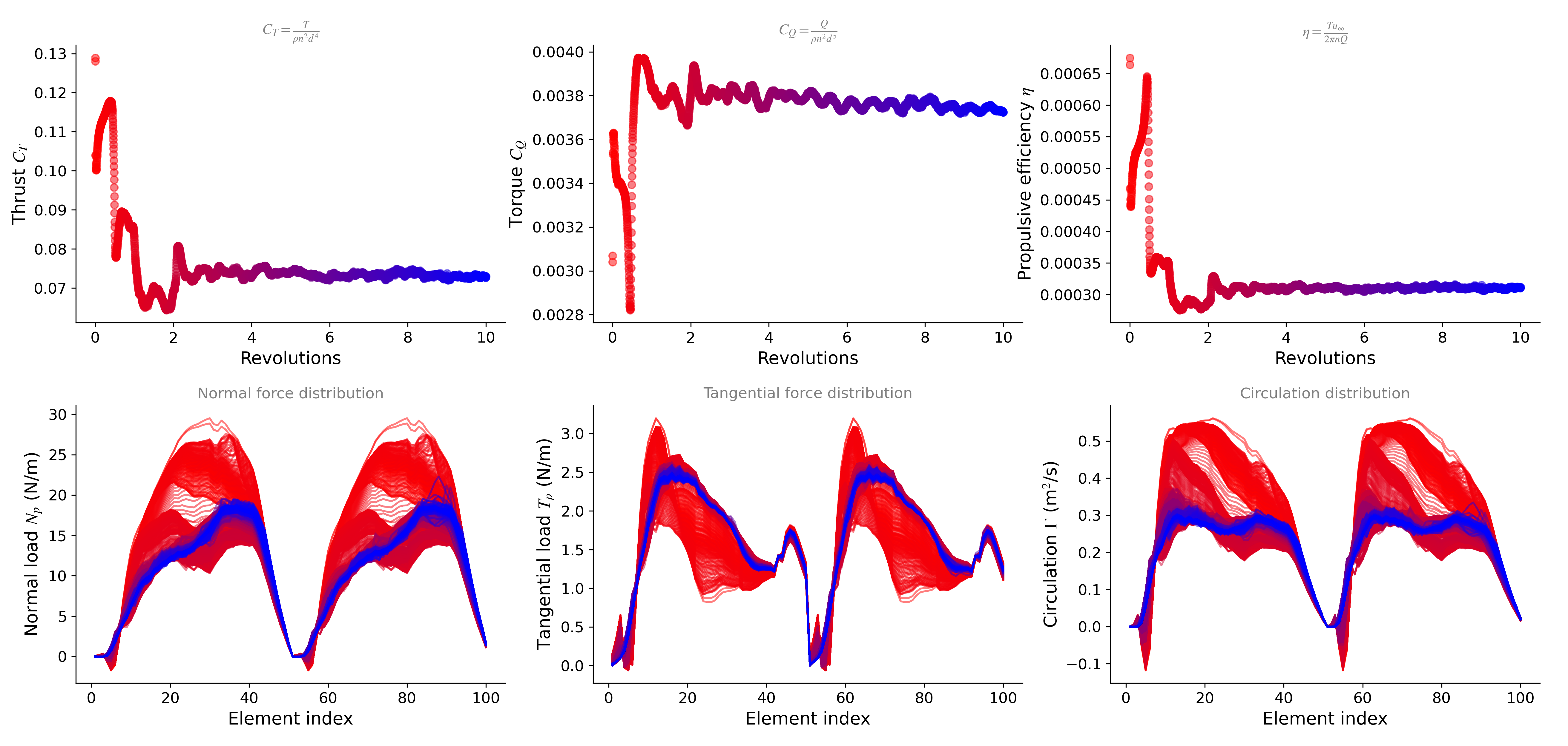
Rotor monitor in the high-fidelity case:
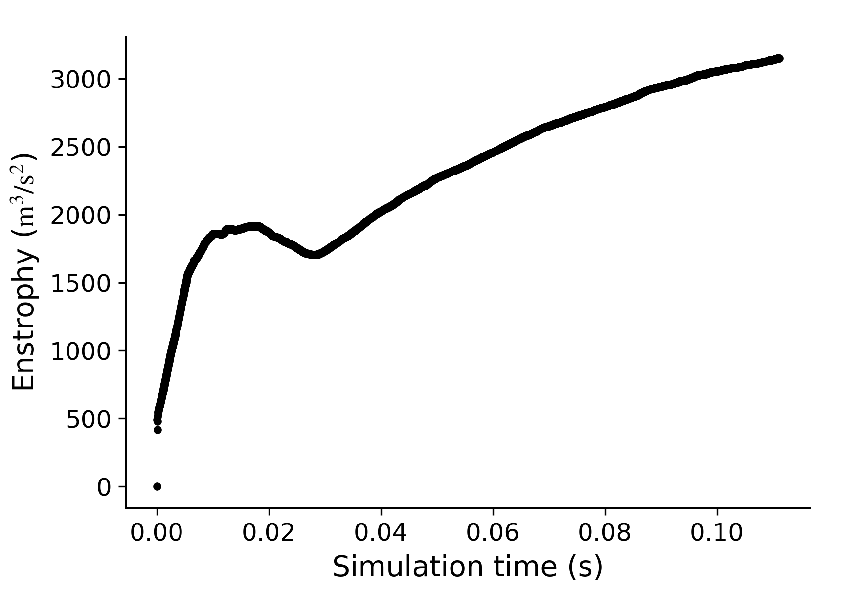
As the simulation runs, you will see the monitor shown below plotting the global enstrophy of the flow. The global enstrophy achieves a steady state once the rate of enstrophy produced by the rotor eventually balances out with the forward scatter of the SFS turbulence model, making the simulation indefinitely stable.
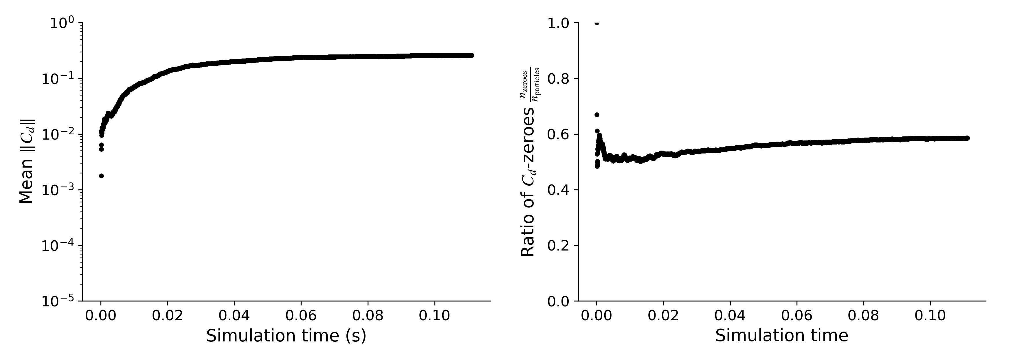
The SFS model uses a dynamic procedure to compute its own model coefficient $C_d$ as the simulation evolves. The value of the model coefficient varies for each particle in space and time. The $C_d$-monitor shown below plots the mean value from all the particle in the field that have a non-zero $C_d$ (left), and also the ratio of the number of particles that got clipped to a zero $C_d$ over the total number of particles (right).
The SFS model helps the simulation to more accurately capture the effects of turbulence from the scales that are not resolved, but it adds computational cost. The following table summarizes the cost of the rVPM, the SFS model, and the $C_d$ dynamic procedure.  The dynamic procedure is the most costly operation, which increases the simulation runtime by about 35%.
If you need to run a case multiple times with only slight changes (e.g., sweeping the AOA and/or RPM), you can first run the simulation with the dynamic procedure (vpm_SFS = vpm.SFS_Cd_twolevel_nobackscatter), take note of what the mean $C_d$ shown in the monitor converges to, and then prescribe that value to subsequent simulations. Prescribing $C_d$ ends up in a simulation that is only 8% slower than the classic VPM without any SFS model.
$C_d$ can then be prescribed as follows
vpm_SFS = vpm.ConstantSFS(vpm.Estr_fmm; Cs=value, clippings=[vpm.clipping_backscatter])where CS = value is the value to prescribe for the model coefficient, and clippings=[vpm.clipping_backscatter] clips the backscatter of enstrophy (making it a purely diffusive model). As a reference, in this hover case, $C_d$ converges to $0.26$ in the high-fidelity simulation.
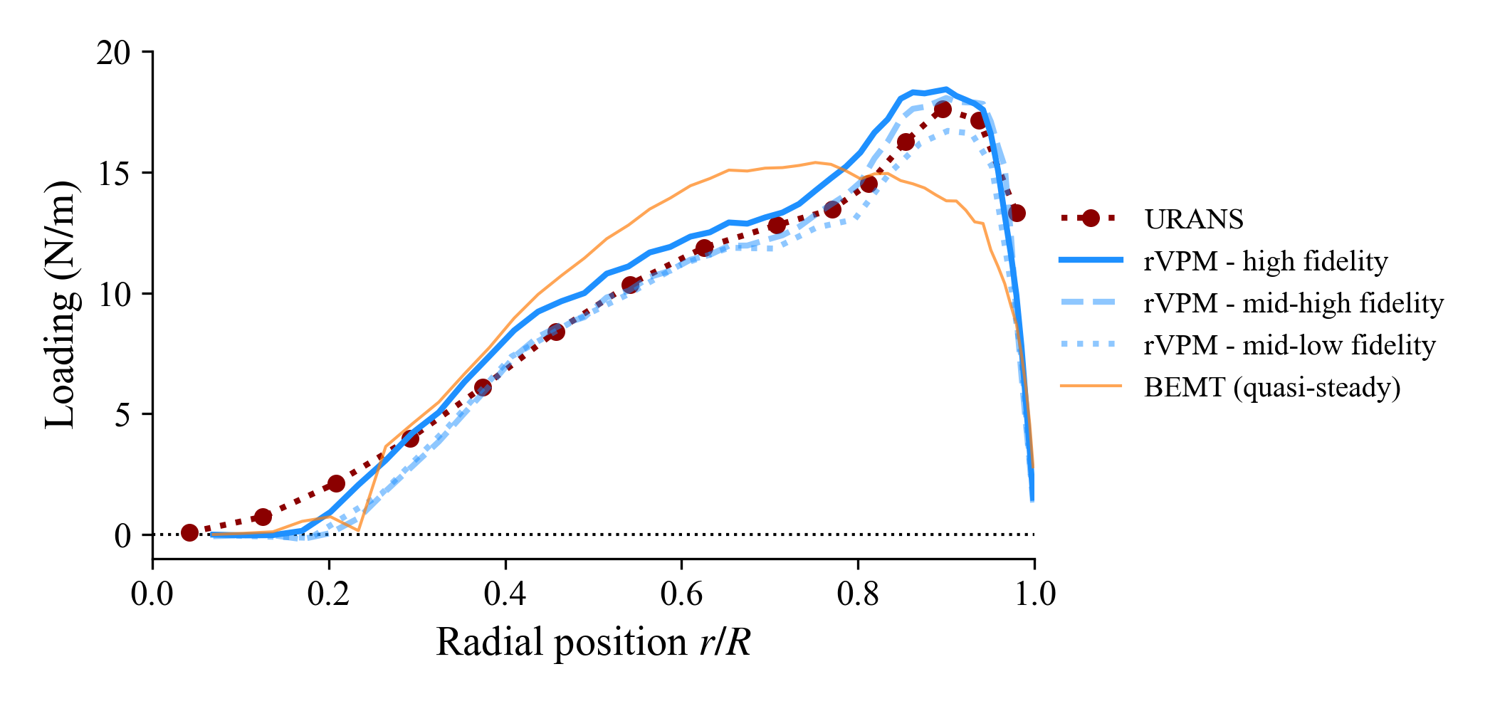
In examples/rotorhover/rotorhover_postprocessing.jl we show how to postprocess the simulations to compare $C_T$ and blade loading to experimental data by Zawodny et al.[1] and a URANS simulation (STAR-CCM+) by Schenk[2]:
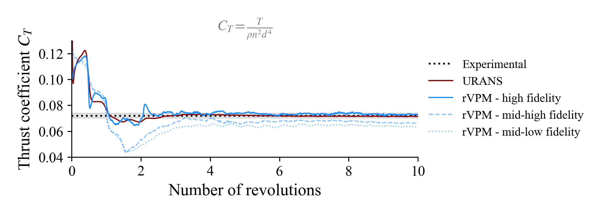
| $C_T$ | Error | |
|---|---|---|
| Experimental | 0.072 | – |
| URANS | 0.071 | 1% |
| rVPM – high fidelity | 0.073 | 1% |
| rVPM – mid-high fidelity | 0.066 | 8% |
| rVPM – mid-low fidelity | 0.064 | 11% |
| BEMT (quasi-steady) | 0.073 | 2% |
In the rotor actuator line model, hub and tip corrections can be applied to $c_\ell$ to account for the effects that bring the aerodynamic loading to zero at the hub and tips. These correction factors, $F_\mathrm{tip}$ and $F_\mathrm{hub}$, are defined as modified Prandtl loss functions,
\[\begin{align*} F_\mathrm{tip} & = \frac{2}{\pi} \cos^{-1} \left( \exp\left( -f_\mathrm{tip} \right) \right) , \qquad f_\mathrm{tip} = \frac{B}{2} \frac{ \left[ \left( \frac{R_\mathrm{rotor}}{r} \right)^{t_1} - 1 \right]^{t_2} }{ \vert \sin \left( \theta_\mathrm{eff} \right) \vert^{t_3} } \\ F_\mathrm{hub} & = \frac{2}{\pi} \cos^{-1} \left( \exp\left( -f_\mathrm{hub} \right) \right) , \qquad f_\mathrm{hub} = \frac{B}{2} \frac{ \left[ \left( \frac{r}{R_\mathrm{hub}} \right)^{h_1} - 1 \right]^{h_2} }{ \vert \sin \left( \theta_\mathrm{eff} \right) \vert^{h_3} } ,\end{align*}\]
where $R_\mathrm{rotor}$ and $R_\mathrm{hub}$ are the rotor and hub radii, $B$ is the number of blades, $r$ is the radial position of the blade element, and $t_1$, $t_2$, $t_3$, $h_1$, $h_2$, and $h_3$ are tunable parameters. The normal and tangential force coefficients, respectively $c_n$ and $c_t$, are then calculated as
\[\begin{align*} c_n & = F_\mathrm{tip} F_\mathrm{hub} c_\ell\cos\theta_\mathrm{eff} + c_d\sin\theta_\mathrm{eff} \\ c_t & = F_\mathrm{tip} F_\mathrm{hub} c_\ell\sin\theta_\mathrm{eff} - c_d\cos\theta_\mathrm{eff} .\end{align*}\]
The hub and tip corrections are passed to uns.run_simulation through the keyword argument hubtiploss_correction = ((t1, t2, t3, tminangle), (h1, h2, h3, hminangle)), where tminangle and hminangle are clipping thresholds for the minimum allowable value of $\vert\theta_\mathrm{eff}\vert$ (in degs) that is used in tip and hub corrections. The following corrections are predefined in FLOWVLM for the user:
import FLOWVLM as vlm

# No corrections
vlm.hubtiploss_nocorrection
((1, 0, Inf, 1.1102230246251565e-15), (1, 0, Inf, 1.1102230246251565e-15))# Original Prandtl corrections
vlm.hubtiploss_correction_prandtl((1, 1, 1, 1.0), (1, 1, 1, 1.0))# Modified Prandtl with a strong hub correction
vlm.hubtiploss_correction_modprandtl((0.6, 5, 0.5, 10), (2, 1, 0.25, 0.05))The .pvsm file visualizing the simulation as shown at the top of this page is available here: LINK (right click → save as...).
To open in ParaView: File → Load State → (select .pvsm file) then select "Search files under specified directory" and point it to the folder where the simulation was saved.
- 1N. S. Zawodny, D. D. Boyd, Jr., and C. L. Burley, “Acoustic Characterization and Prediction of Representative, Small-scale Rotary-wing Unmanned Aircraft System Components,” in 72nd American Helicopter Society (AHS) Annual Forum (2016).
- 2A. R. Schenk, "Computational Investigation of the Effects of Rotor-on-Rotor Interactions on Thrust and Noise," Masters thesis, Brigham Young University (2020).