Aeroacoustic Noise
Using the aerodynamic solution obtained in the previous section, we can now feed the time-resolved loading and blade motion to PSU-WOPWOP and BPM.jl to compute aeroacoustic noise. PSU-WOPWOP is a Ffowcs Williams-Hawkings acoustic analogy using the time-domain integral Farassat 1A formulation to compute tonal noise from loading and thickness sources (FLOWUnsteady uses a compact representation for the loading source, while using the actual 3D loft of the blade for the thickness source). BPM.jl is an implementation of the semi-empirical methodology developed by Brooks, Pope, and Marcolini to predict broadband noise. The methodology models five self-noise mechanisms due to boundary-layer phenomena: boundary-layer turbulence passing the trailing edge, separated boundary-layer and stalled-airfoil flow, vortex shedding due to laminar-boundary-layer instabilities, vortex shedding from blunt trailing edges, and turbulent flow due to vortex tip formation.
In the following code we exemplify the following:
- How to define observers (microphones) to probe the aeroacoustic noise
- How to call PSU-WOPWOP through
uns.run_noise_wopwop - How to call BPM.jl through
uns.run_noise_bpm - How to add the tonal and broadband noise together and postprocess
As a reference, this is the orientation of the rotor and microphone array used in this example:
PSU-WOPWOP is a closed-source code that is not included in FLOWUnsteady, but is graciously made available as a binary by its developers at Penn State University upon inquiry. We recommend contacting them directly to obtain a binary.
FLOWUnsteady has been tested with PSU-WOPWOP v3.4.4.
Preamble
We load FLOWUnsteady and the FLOWUnsteady.noise module:
import FLOWUnsteady as uns
import FLOWUnsteady: gt, vlm, noise

# Path where to read and save simulation data
sims_path = "/media/edoalvar/T7/simulationdata202304"
Tonal Noise
First, we calculate the tonal noise from loading and thickness sources. The loading of each blade is read from each time step of the the aerodynamic solution, which is an unsteady loading. The thickness is computed from the 3D lofted geometry that is also outputted by the aero solution.
These files are read calling uns.run_noise_wopwop, which converts the outputs of the aero solution into a PSU-WOPWOP case. The PSU-WOPWOP binary is then called to read the case and propagate the noise to a set of observers (microphones). The PSU-WOPWOP solution is then written to the same case folder.
# Path from where to read aerodynamic solution
read_path       = joinpath(sims_path, "rotorhover-example-midhigh00") # <-- This must point to you aero simulation

# Path where to save PSU-WOPWOP outputs
save_ww_path    = read_path*"-pww/"

# Path to PSU-WOPWOP binary (not included in FLOWUnsteady)
wopwopbin       = "/home/edoalvar/Dropbox/WhisperAero/OtherCodes/PSU-WOPWOP_v3.4.4/wopwop3_linux_serial"

# Run name (prefix of rotor files to read)
run_name        = "singlerotor"

# Make this `true` if the aero simulation used the quasi-steady solver. If so,
# PSU-WOPWOP will assume that the blade loading and geometry stays constant
# and will read only one step out of the aero solution
const_solution  = false

# ------------ PARAMETERS ------------------------------------------------------
# NOTE: Make sure that these parameters match what was used in the
#       aerodynamic solution

# Rotor geometry
rotor_file      = "DJI9443.csv"        # Rotor geometry
data_path       = uns.def_data_path    # Path to rotor database

# Read radius of this rotor and number of blades
R, B            = uns.read_rotor(rotor_file; data_path=data_path)[[1,3]]

rotorsystems    = [[B]]                # rotorsystems[si][ri] is the number of blades of the ri-th rotor in the si-th system

# Simulation parameters
RPM             = 5400                 # RPM here is a reference value to go from nrevs to simulation time
CW              = false                # Clock-wise rotation of constant geometry (used if const_solution=true)
rho             = 1.071778             # (kg/m^3) air density
speedofsound    = 342.35               # (m/s) speed of sound

# Aero input parameters
nrevs           = 2                    # Number of revolutions to read
nrevs_min       = 6                    # Start reading from this revolution
nsteps_per_rev  = 72                   # Number of steps per revolution in aero solution
num_min         = ceil(Int, nrevs_min*nsteps_per_rev) # Start reading aero files from this step number

if const_solution                       # If constant solution, it overrides to read only the first time step
    nrevs       = nothing
    nsteps_per_rev = nothing
    num_min     = 1
end


# PSU-WOPWOP parameters
ww_nrevs        = 18                     # Number of revolutions in PSU-WOPWOP (18 revs at 5400 RPM gives fbin = 5 Hz)
ww_nsteps_per_rev = max(120, 2*nsteps_per_rev) # Number of steps per revolution in PSU-WOPWOP
const_geometry  = const_solution       # Whether to run PSU-WOPWOP on constant geometry read from num_min
periodic        = true                 # Periodic aerodynamic solution
highpass        = 0.0                  # High pass filter (set this to >0 to get rid of 0th freq in OASPL)

# NOTE: `periodic=true` assumes that the aero solution is periodic, which allows
#       PSU-WOPWOP to simulate more revolutions (`ww_nrevs`) that what is
#       read from the aero simulation (`nrevs`). This is a good assumption for
#       an unsteady simulation as long as the loading is somewhat periodic after
#       the initial transient state (even with small unsteady fluctuations),
#       but set it to `false` in simulations with complex control inputs
#       (e.g., maneuvering aircraft, variable RPM, etc). If the outputs of
#       PSU-WOPWOP seem nonsensical, try setting this to false and increasing
#       the number of revolutions in the aero solution (`nrevs`).


# Observer definition: Circular array of microphones
sph_R           = 1.905                # (m) radial distance from rotor hub
sph_nR          = 0                    # Number of microphones in the radial direction
sph_nphi        = 0                    # Number of microphones in the zenith direction
sph_ntht        = 72                   # Number of microphones in the azimuthal direction
sph_thtmin      = 0                    # (deg) first microphone's angle
sph_thtmax      = 360                  # (deg) last microphone's angle
sph_phimax      = 180
sph_rotation    = [90, 0, 0]           # Rotation of grid of microphones

# NOTE: Here we have defined the microphone array as a circular array, but
#       we could have defined a hemisphere instead by simply making `sph_nphi`
#       different than zero, or a full volumetric spherical mesh making `sph_nR`
#       different than zero

# Alternative observer definition: Single microphone
Rmic            = 1.905                # (m) radial distance from rotor hub
anglemic        = 90*pi/180            # (rad) microphone angle from plane of rotation (- below, + above)
                                       # 0deg is at the plane of rotation, 90deg is upstream
microphoneX     = nothing              # Comment and uncomment this to switch from array to single microphone
# microphoneX   = Rmic*[-sin(anglemic), cos(anglemic), 0]


# ------------ RUN PSU-WOPWOP ----------------------------------------------
@time uns.run_noise_wopwop(read_path, run_name, RPM, rho, speedofsound, rotorsystems,
                            ww_nrevs, ww_nsteps_per_rev, save_ww_path, wopwopbin;
                            nrevs=nrevs, nsteps_per_rev=nsteps_per_rev,
                            # ---------- OBSERVERS -------------------------
                            sph_R=sph_R,
                            sph_nR=sph_nR, sph_ntht=sph_ntht,
                            sph_nphi=sph_nphi, sph_phimax=sph_phimax,
                            sph_rotation=sph_rotation,
                            sph_thtmin=sph_thtmin, sph_thtmax=sph_thtmax,
                            microphoneX=microphoneX,
                            # ---------- SIMULATION OPTIONS ----------------
                            periodic=periodic,
                            # ---------- INPUT OPTIONS ---------------------
                            num_min=num_min,
                            const_geometry=const_geometry,
                            axisrot="automatic",
                            CW=CW,
                            highpass=highpass,
                            # ---------- OUTPUT OPTIONS --------------------
                            verbose=true, v_lvl=0,
                            prompt=true, debug_paraview=false,
                            debuglvl=0,                     # PSU-WOPWOP debug level (verbose)
                            observerf_name="observergrid",  # .xyz file with observer grid
                            case_name="runcase",            # Name of case to create and run
                            );
The length of the frequency bins in the SPL spectrum obtained from the FFT falls out from the following relationships
\[\begin{align*} f_\mathrm{bin} = \frac{f_\mathrm{sample}}{n_\mathrm{samples}} = \frac{1}{n_\mathrm{samples} \Delta t_\mathrm{sample}} = \frac{\mathrm{RPM}}{60}\frac{1}{n_\mathrm{revs}} .\end{align*}\]
Thus, in order to obtain the desired frequency bin $f_\mathrm{bin}$, the number of revolutions that PSU-WOPWOP needs to simulate (ww_nrevs) is
\[\begin{align*} n_\mathrm{revs} = \frac{\mathrm{RPM}}{60}\frac{1}{f_\mathrm{bin}} .\end{align*}\]
If you need to debug the aero→acoustics workflow, it is useful to convert the input files that we gave to PSU-WOPWOP back to VTK and visualize them in ParaView. This helps verify that we are passing the right things to PSU-WOPWOP. The following lines grab those input files that are formated for PSU-WOPWOP, converts them into VTK files, and opens them in ParaView:
read_ww_path   = joinpath(save_ww_path, "runcase")      # Path to PWW's input files
save_vtk_path  = joinpath(read_ww_path, "vtks")         # Where to save VTK files

# Generate VTK files
vtk_str = noise.save_geomwopwop2vtk(read_ww_path, save_vtk_path)

println("Generated the following files:\n\t$(vtk_str)")

# Call Paraview to visualize VTKs
run(`paraview --data=$(vtk_str)`)
Broadband Noise
Now, we calculate the broadband noise from non-deterministic sources through BPM. This is done calling uns.run_noise_bpm as follows:
# Path where to save BPM outputs
save_bpm_path   = joinpath(sims_path, "rotorhover-example-midhigh00-bpm")

# ------------ PARAMETERS --------------------------------------------------
# NOTE: Make sure that these parameters match what was used in the
#       aerodynamic solution

# Rotor geometry
rotor_file      = "DJI9443.csv"        # Rotor geometry
data_path       = uns.def_data_path    # Path to rotor database
read_polar      = vlm.ap.read_polar2   # What polar reader to use
pitch           = 0.0                  # (deg) collective pitch of blades
n               = 50                   # Number of blade elements (this does not need to match the aero solution)
CW              = false                # Clock-wise rotation

# Read radius of this rotor and number of blades
R, B            = uns.read_rotor(rotor_file; data_path=data_path)[[1,3]]

# Simulation parameters
RPM             = 5400                 # RPM
J               = 0.0001               # Advance ratio Vinf/(nD)
AOA             = 0                    # (deg) Angle of attack (incidence angle)

rho             = 1.071778             # (kg/m^3) air density
mu              = 1.85508e-5           # (kg/ms) air dynamic viscosity
speedofsound    = 342.35               # (m/s) speed of sound

magVinf         = J*RPM/60*(2*R)
Vinf(X,t)       = magVinf*[cosd(AOA), sind(AOA), 0]  # (m/s) freestream velocity

# BPM parameters
TE_thickness    = 16.0                 # (deg) trailing edge thickness
noise_correction= 1.00                 # Calibration parameter (1 = no correction)
freq_bins       = uns.BPM.default_f    # Frequency bins (default is one-third octave band)

# Observer definition: Circular array of microphones
sph_R           = 1.905                # (m) radial distance from rotor hub
sph_nR          = 0                    # Number of microphones in the radial direction
sph_nphi        = 0                    # Number of microphones in the zenith direction
sph_thtmin      = 0                    # (deg) first microphone's angle
sph_thtmax      = 360                  # (deg) last microphone's angle
sph_phimax      = 180
sph_rotation    = [90, 0, 0]           # Rotation of grid of microphones

# Alternative observer definition: Single microphone
Rmic            = 1.905                # (m) radial distance from rotor hub
anglemic        = 90*pi/180            # (rad) microphone angle from plane of rotation (- below, + above)
                                       # 0deg is at the plane of rotation, 90deg is upstream
microphoneX     = nothing              # Comment and uncomment this to switch from array to single microphone
# microphoneX   = Rmic*[-sin(anglemic), cos(anglemic), 0]

# ------------ GENERATE GEOMETRY -------------------------------------------
# Generate rotor
rotor = uns.generate_rotor(rotor_file; pitch=pitch,
                                        n=n, CW=CW, ReD=0.0,
                                        verbose=false, xfoil=false,
                                        data_path=data_path,
                                        read_polar=read_polar,
                                        plot_disc=false)

rotors = vlm.Rotor[rotor]              # All rotors in the computational domain

# ------------ RUN BPM -----------------------------------------------------
uns.run_noise_bpm(rotors, RPM, Vinf, rho, mu, speedofsound,
                                save_bpm_path;
                                # ---------- OBSERVERS -------------------------
                                sph_R=sph_R,
                                sph_nR=sph_nR, sph_ntht=sph_ntht,
                                sph_nphi=sph_nphi, sph_phimax=sph_phimax,
                                sph_rotation=sph_rotation,
                                sph_thtmin=sph_thtmin, sph_thtmax=sph_thtmax,
                                microphoneX=microphoneX,
                                # ---------- BPM OPTIONS -----------------------
                                noise_correction=noise_correction,
                                TE_thickness=TE_thickness,
                                freq_bins=freq_bins,
                                # ---------- OUTPUT OPTIONS --------------------
                                prompt=true
                                );
Results
Finally, we add tonal and broadband noise together and plot the results
Read datasets
We start by reading the outputs from PSU-WOPWOP and BPM:
# Dataset to read and associated information
dataset_infos = [ # (label, PWW solution, BPM solution, line style, color)
                    ("FLOWUnsteady",
                        joinpath(sims_path, "rotorhover-example-midhigh00-pww/runcase/"),
                        joinpath(sims_path, "rotorhover-example-midhigh00-bpm"),
                        "-", "steelblue"),
                ]

datasets_pww = Dict()     # Stores PWW data in this dictionary
datasets_bpm = Dict()     # Stores BPM data in this dictionary

# Read datasets and stores them in dictionaries
noise.read_data(dataset_infos; datasets_pww=datasets_pww, datasets_bpm=datasets_bpm)

println("Done!")
Also, we need to recreate the circular array of microphones that was used when generating the aeroacoustic solutions:
# These parameters will be used for plotting
RPM          = 5400                  # RPM of solution
nblades      = 2                     # Number of blades
BPF          = nblades*RPM/60        # Blade passing frequency

# Make sure this grid is the same used as an observer by the aeroacoustic solution
sph_R        = 1.905                 # (m) radial distance from rotor hub
sph_nR       = 0
sph_nphi     = 0
sph_ntht     = 72                    # Number of microphones
sph_thtmin   = 0                     # (deg) first microphone's angle
sph_thtmax   = 360                   # (deg) last microphone's angle
sph_phimax   = 180
sph_rotation = [90, 0, 0]            # Rotation of grid of microphones

# Create observer grid
grid = noise.observer_sphere(sph_R, sph_nR, sph_ntht, sph_nphi;
                                thtmin=sph_thtmin, thtmax=sph_thtmax, phimax=sph_phimax,
                                rotation=sph_rotation);

# This function calculates the angle that corresponds to every microphone
pangle(i) = -180/pi*atan(gt.get_node(grid, i)[1], gt.get_node(grid, i)[2])
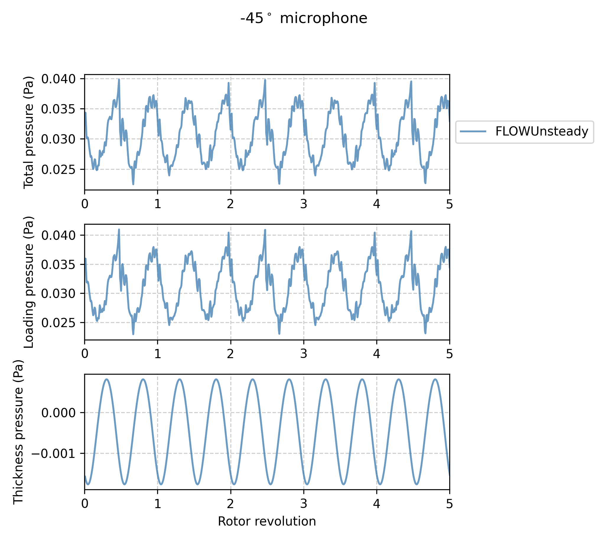
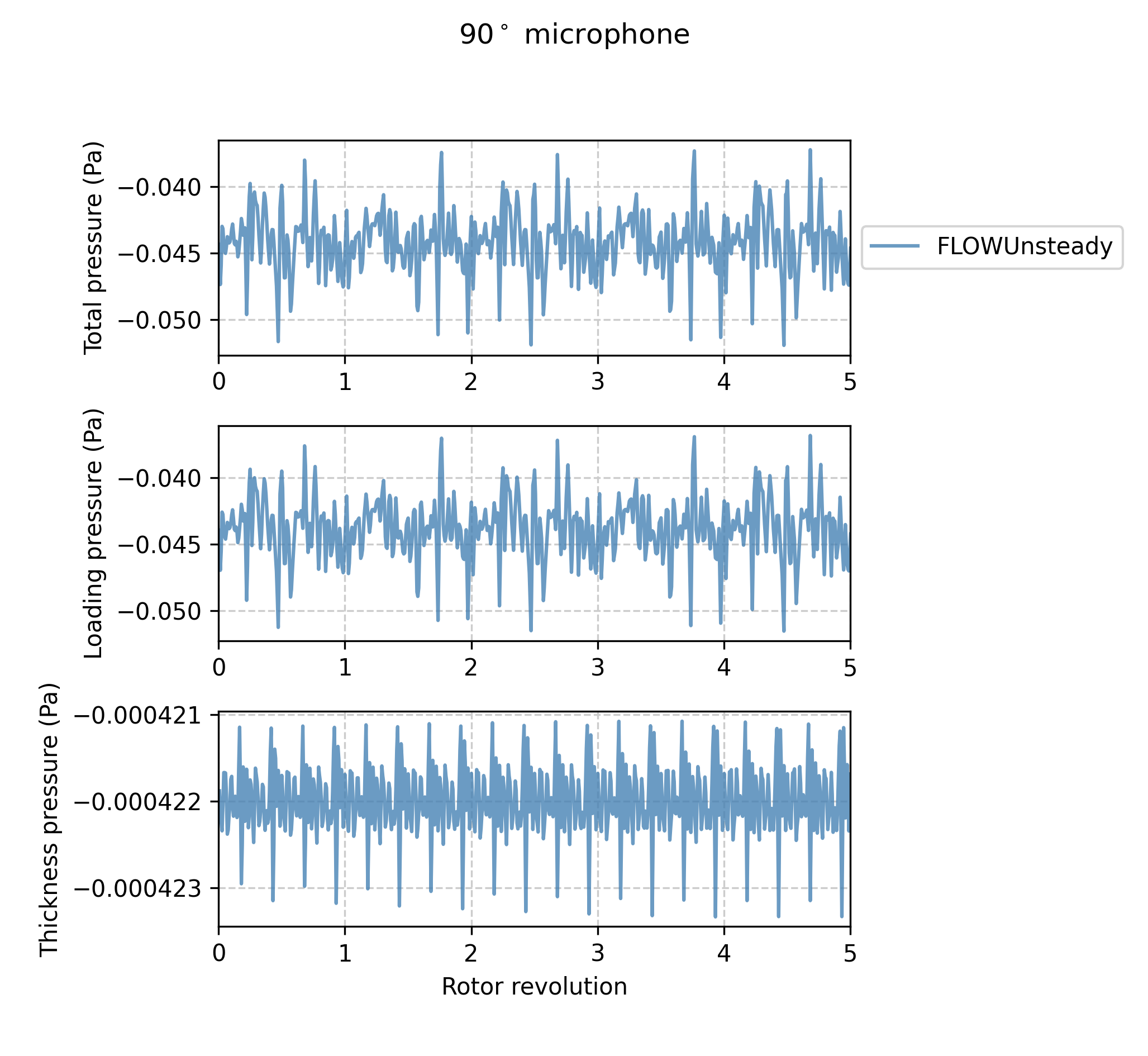
Pressure waveform
Here we plot the pressure waveform at some of the microphones. This pressure waveform includes only the tonal component, as given by PSU-WOPWOP.
microphones  = [-45, 90]            # (deg) microphones to plot

noise.plot_pressure(dataset_infos, microphones, RPM, sph_ntht, pangle;
                                datasets_pww=datasets_pww, xlims=[0, 5])
SPL Spectrum
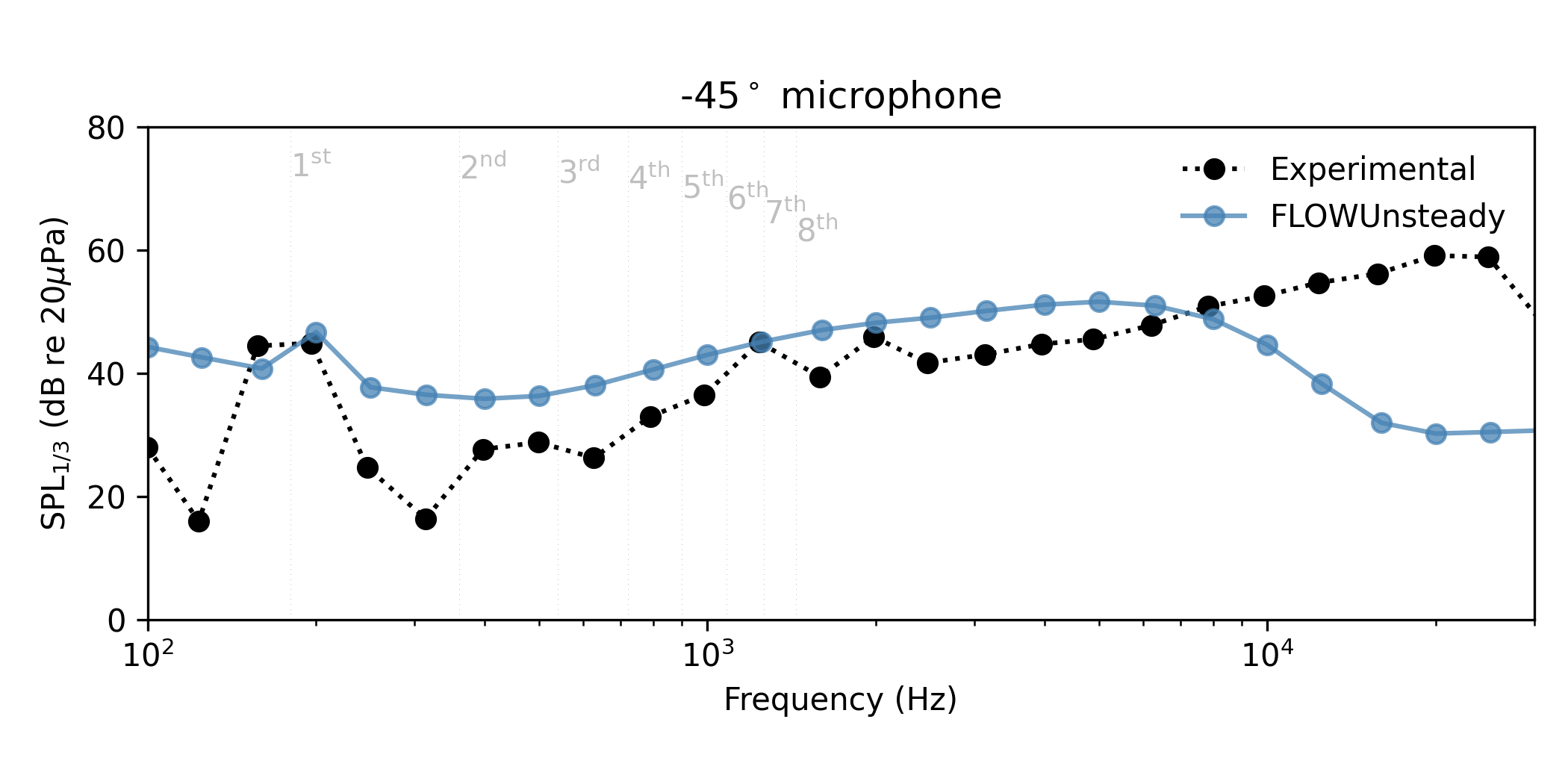
We now compare the (sound pressure level) SPL spectrum at the microphone $-45^\circ$ below the plane of rotation with the experimental data reported by Zawodny et al.[1].
One-third octave band:
microphones  = [-45]                # (deg) microphone to plot
Aweighted    = false                # Plot A-weighted SPL
onethirdoctave = true               # Plot 1/3 octave band

# Experimental data from Zawodny et al., Fig. 9
zawodny_path = joinpath(uns.examples_path, "..", "docs", "resources", "data", "zawodny2016")
exp_filename = joinpath(zawodny_path, "zawodny_dji9443-fig9-OTO-5400.csv")
plot_experimental = [(exp_filename, "Experimental", "o:k", Aweighted, [])]

# Plot SPL spectrum
noise.plot_spectrum_spl(dataset_infos, microphones, BPF, sph_ntht, pangle;
                          datasets_pww=datasets_pww, datasets_bpm=datasets_bpm,
                          Aweighted=Aweighted,
                          onethirdoctave=onethirdoctave,
                          plot_csv=plot_experimental,
                          xBPF=false, xlims=[100, 3e4], ylims=[0, 80], BPF_lines=8)
A-weighted narrow band:
Aweighted    = true                # Plot A-weighted SPL

# Experimental data from Zawodny et al., Fig. 9
exp_filename = joinpath(zawodny_path, "zawodny_dji9443_spl_5400_01.csv")
plot_experimental = [(exp_filename, "Experimental", "k", Aweighted, [])]

# Plot SPL spectrum
noise.plot_spectrum_spl(dataset_infos, microphones, BPF, sph_ntht, pangle;
                          datasets_pww=datasets_pww, datasets_bpm=datasets_bpm,
                          Aweighted=Aweighted,
                          plot_csv=plot_experimental,
                          xBPF=false, xlims=[100, 3e4], BPF_lines=21)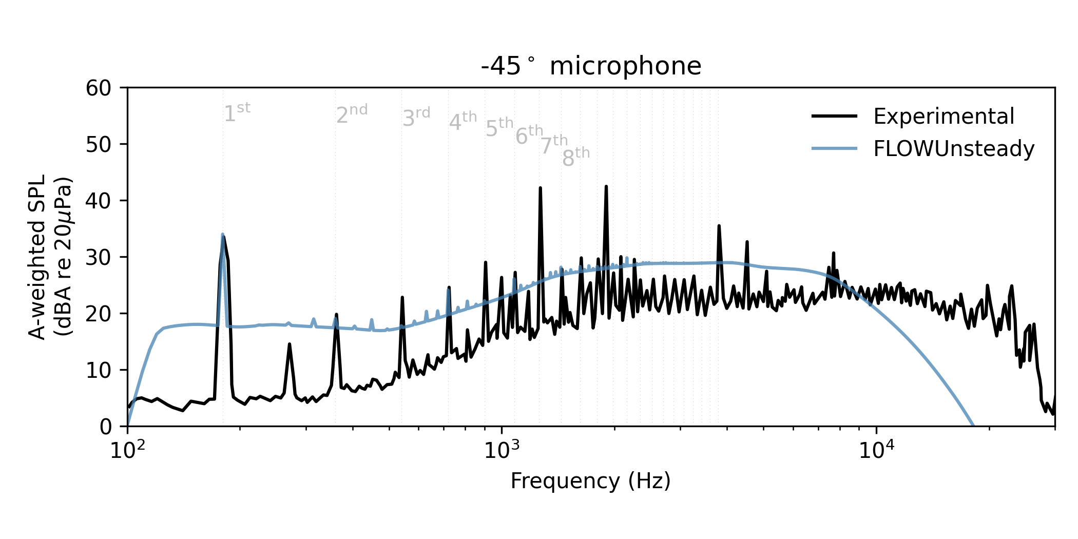
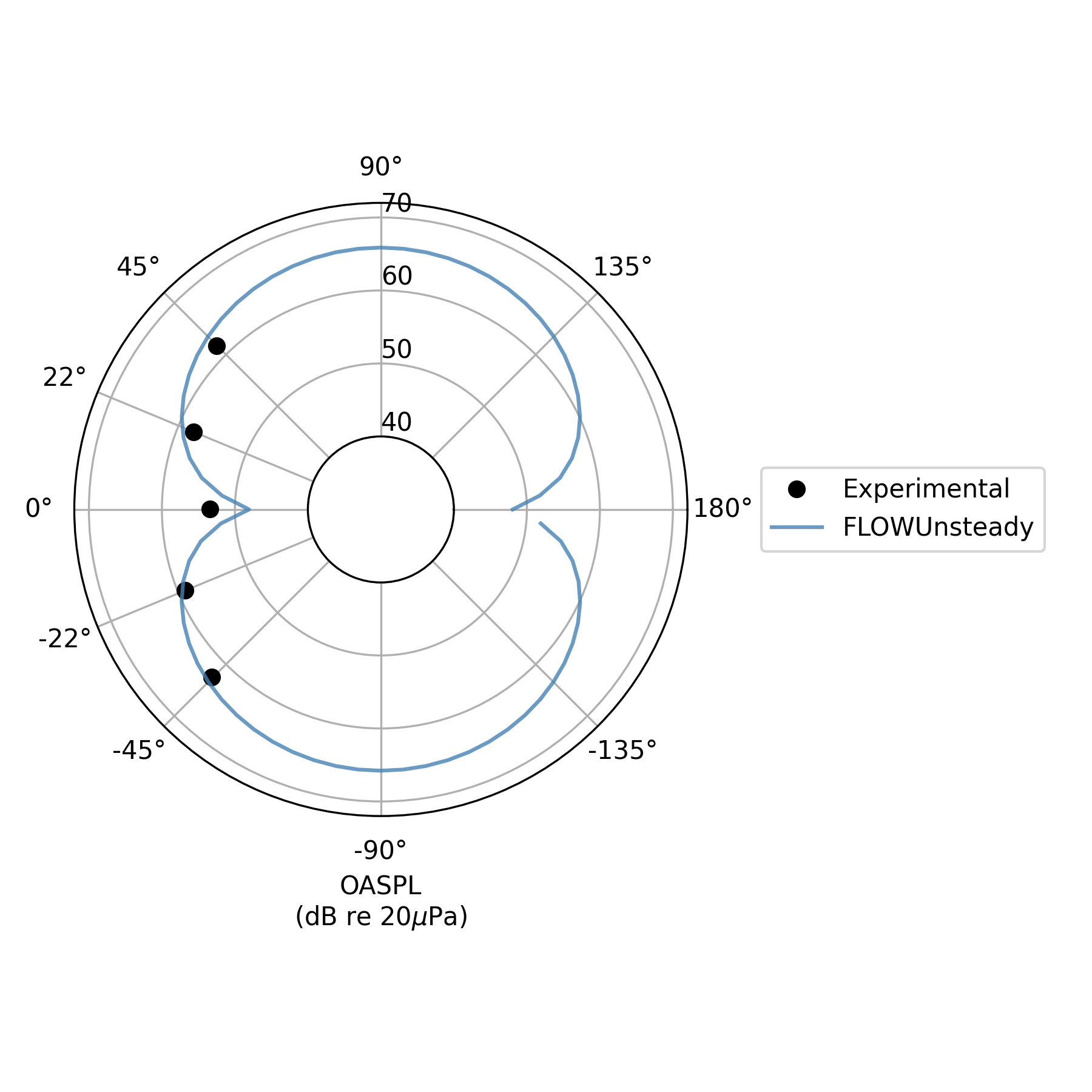
In the narrow band spectrum, keep in mind that the broadband output of BPM has been converted from 1/3 octaves into narrow band (5 hz bin) in order to plot it together with the tonal noise, but this is a very rough approximation (we lack enough information to interpolate from a coarse band to a narrow band besides just smearing the energy content). Hence, the broadband component seems to overpredict relative to the experimental, but this is an artifice of the 1/3 octave $\rightarrow$ narrow band conversion. In the OASPL directivity plots we will see that the A-weighted OASPL predicted with BPM actually matches the experimental values very well.
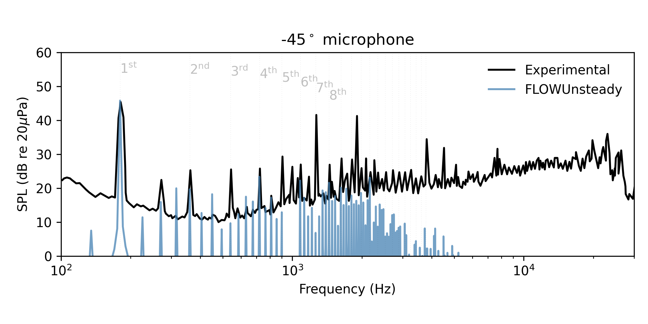
Tonal noise
Here we plot only the tonal component of noise associated with harmonics of the blade passing frequency (BPF),
Tonal SPL spectrum
Aweighted       = false
add_broadband   = false

# Experimental data from Zawodny et al., Fig. 9
exp_filename = joinpath(zawodny_path, "zawodny_dji9443_spl_5400_01.csv")
plot_experimental = [(exp_filename, "Experimental", "k", Aweighted, [])]

# Plot SPL spectrum
noise.plot_spectrum_spl(dataset_infos, microphones, BPF, sph_ntht, pangle;
                          datasets_pww=datasets_pww, datasets_bpm=datasets_bpm,
                          Aweighted=Aweighted,
                          plot_csv=plot_experimental,
                          add_broadband=add_broadband,
                          xBPF=false, xlims=[100, 3e4], BPF_lines=21)
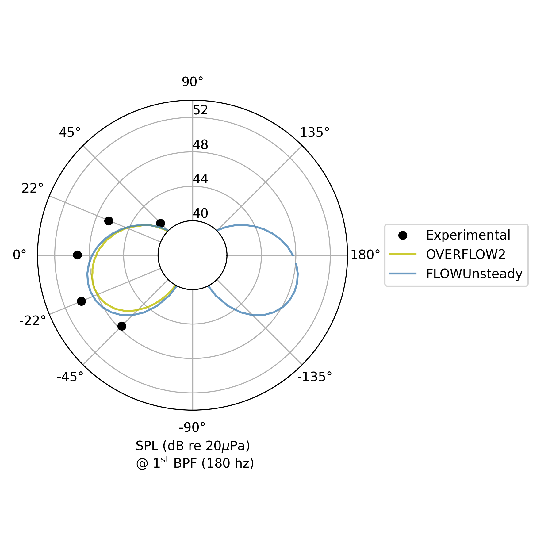
Directivity of $1^\mathrm{st}$ BPF
BPFi = 1                 # Multiple of blade-passing frequency to plot

# Experimental and computational data reported by Zawodny et al., Fig. 14
filename1 = joinpath(zawodny_path, "zawodny_fig14_topright_exp00.csv")
filename2 = joinpath(zawodny_path, "zawodny_fig14_topright_of00.csv")
filename3 = joinpath(zawodny_path, "zawodny_fig14_topright_pas00.csv")

plot_experimental = [(filename1, "Experimental", "ok", Aweighted, []),
                     (filename2, "OVERFLOW2", "-y", Aweighted, [(:alpha, 0.8)])]

# Plot SPL directivity of first blade-passing frequency
noise.plot_directivity_splbpf(dataset_infos, BPFi, BPF, pangle;
                                    datasets_pww=datasets_pww,
                                    datasets_bpm=datasets_bpm,
                                    plot_csv=plot_experimental,
                                    rticks=40:4:52, rlims=[40, 54], rorigin=36)
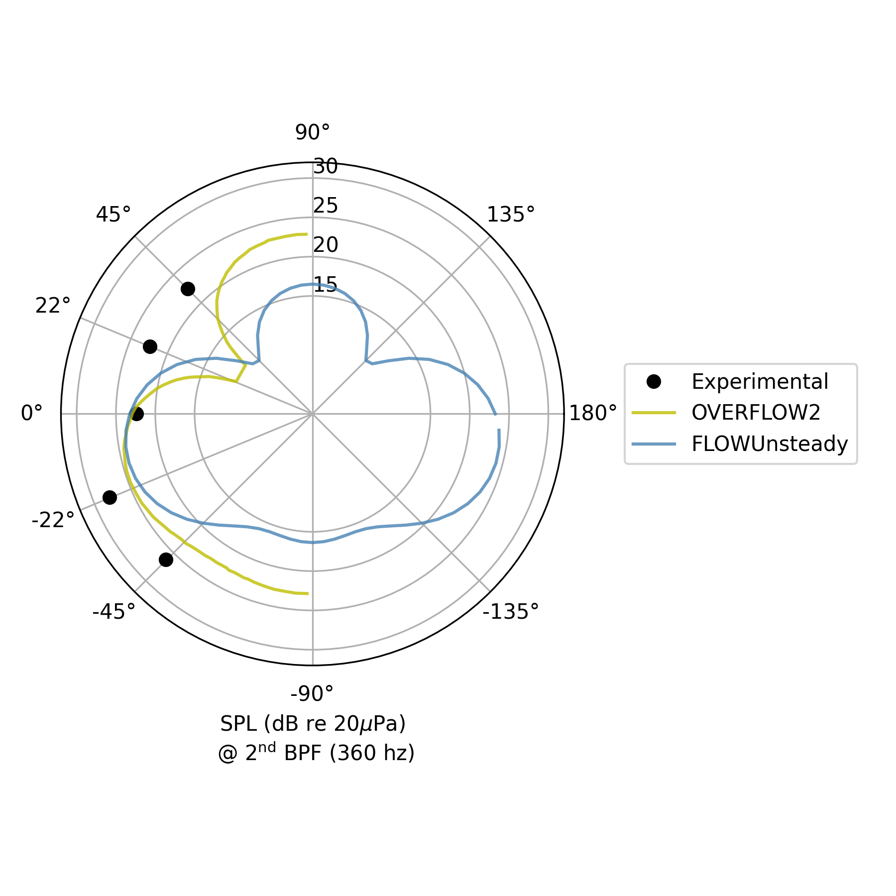
Directivity of $2^\mathrm{nd}$ BPF
BPFi = 2                 # Multiple of blade-passing frequency to plot

# Experimental and computational data reported by Zawodny et al., Fig. 14
filename1 = joinpath(zawodny_path, "zawodny_fig14_bottomright_exp00.csv")
filename2 = joinpath(zawodny_path, "zawodny_fig14_bottomright_of00.csv")
filename3 = joinpath(zawodny_path, "zawodny_fig14_bottomright_pas00.csv")

plot_experimental = [(filename1, "Experimental", "ok", Aweighted, []),
                     (filename2, "OVERFLOW2", "-y", Aweighted, [(:alpha, 0.8)])]

# Plot SPL directivity of first blade-passing frequency
noise.plot_directivity_splbpf(dataset_infos, BPFi, BPF, pangle;
                                    datasets_pww=datasets_pww,
                                    datasets_bpm=datasets_bpm,
                                    plot_csv=plot_experimental,
                                    rticks=15:5:30, rlims=[0, 32], rorigin=0)
OASPL directivity
Unweighted overall SPL (OASPL)
Aweighted = false

# Experimental and computational data reported by Zawodny et al., Fig. 12
exp_filename = joinpath(zawodny_path, "zawodny_fig12_left_5400_00.csv")
plot_experimental = [(exp_filename, "Experimental", "ok", Aweighted, [])]

# Plot OASPL directivity
noise.plot_directivity_oaspl(dataset_infos, pangle;
                                    datasets_pww=datasets_pww,
                                    datasets_bpm=datasets_bpm,
                                    Aweighted=Aweighted,
                                    plot_csv=plot_experimental,
                                    rticks=40:10:70, rlims=[40, 72], rorigin=30)
A-weighted OASPL
Aweighted = true

# Experimental and computational data reported by Zawodny et al., Fig. 12
exp_filename = joinpath(zawodny_path, "zawodny_fig12_right_5400_00.csv")
plot_experimental = [(exp_filename, "Experimental", "ok", Aweighted, [])]

# Plot OASPL directivity
noise.plot_directivity_oaspl(dataset_infos, pangle;
                                    datasets_pww=datasets_pww,
                                    datasets_bpm=datasets_bpm,
                                    Aweighted=Aweighted,
                                    plot_csv=plot_experimental,
                                    rticks=40:10:70, rlims=[40, 72], rorigin=30)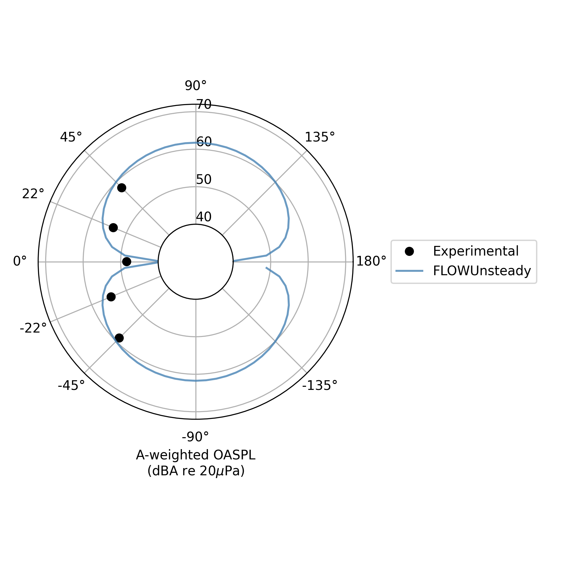
- 1N. S. Zawodny, D. D. Boyd, Jr., and C. L. Burley, “Acoustic Characterization and Prediction of Representative, Small-scale Rotary-wing Unmanned Aircraft System Components,” in 72nd American Helicopter Society (AHS) Annual Forum (2016).