Basics
In this example we first simulate an APC Thin-Electric 10x7 propeller operating in cruise conditions. Along the way, we demonstrate the basics of how to set up and run a rotor simulation.
Rotors are generated through the function FLOWUnsteady.generate_rotor, which can receive either a set of parameters that define the rotor geometry (like twist/chord/sweep distributions, etc), or it can read the rotor geometry from a file. FLOWunsteady provides a prepopulated database of airfoil and rotor geometries to automate the generation of rotors, which is found under database/. This database can be accessed through the variable FLOWUnsteady.default_database. Alternatively, users can define their own database with custom rotors and airfoils.
The following slides describe the structure of the database, using a DJI rotor as an example:
In this simulation we exemplify the following:
- How to generate a rotor with
uns.generate_rotor - How to generate a rotor monitor with
uns.generate_monitor_rotors - How to set up and run a rotor simulation.
#=##############################################################################
# DESCRIPTION
    Simulation of an APC Thin-Electric 10x7 propeller (two-bladed rotor, 10-inch
    diameter).

    This example replicates the experiment and simulation described in McCrink &
    Gregory (2017), "Blade Element Momentum Modeling of Low-Reynolds Electric
    Propulsion Systems."

# AUTHORSHIP
  * Author          : Eduardo J. Alvarez (edoalvarez.com)
  * Email           : Edo.AlvarezR@gmail.com
  * Created         : Mar 2023
  * Last updated    : Mar 2023
  * License         : MIT
=###############################################################################

import FLOWUnsteady as uns
import FLOWVLM as vlm
import FLOWVPM as vpm

run_name        = "propeller-example"       # Name of this simulation

save_path       = run_name                  # Where to save this simulation
paraview        = true                      # Whether to visualize with Paraview


# ----------------- GEOMETRY PARAMETERS ----------------------------------------

# Rotor geometry
rotor_file      = "apc10x7.csv"             # Rotor geometry
data_path       = uns.def_data_path         # Path to rotor database
pitch           = 0.0                       # (deg) collective pitch of blades
CW              = false                     # Clock-wise rotation
xfoil           = true                      # Whether to run XFOIL
ncrit           = 9                         # Turbulence criterion for XFOIL

# NOTE: If `xfoil=true`, XFOIL will be run to generate the airfoil polars used
#       by blade elements before starting the simulation. XFOIL is run
#       on the airfoil contours found in `rotor_file` at the corresponding
#       local Reynolds and Mach numbers along the blade.
#       Alternatively, the user can provide pre-computer airfoil polars using
#       `xfoil=false` and pointing to polar files through `rotor_file`.

# Discretization
n               = 20                        # Number of blade elements per blade
r               = 1/5                       # Geometric expansion of elements

# NOTE: Here a geometric expansion of 1/5 means that the spacing between the
#       tip elements is 1/5 of the spacing between the hub elements. Refine the
#       discretization towards the blade tip like this in order to better
#       resolve the tip vortex.

# Read radius of this rotor and number of blades
R, B            = uns.read_rotor(rotor_file; data_path=data_path)[[1,3]]

# ----------------- SIMULATION PARAMETERS --------------------------------------

# Operating conditions
RPM             = 9200                      # RPM
J               = 0.4                       # Advance ratio Vinf/(nD)
AOA             = 0                         # (deg) Angle of attack (incidence angle)

rho             = 1.225                     # (kg/m^3) air density
mu              = 1.81e-5                   # (kg/ms) air dynamic viscosity
speedofsound    = 342.35                    # (m/s) speed of sound

magVinf         = J*RPM/60*(2*R)
Vinf(X, t)      = magVinf*[cosd(AOA), sind(AOA), 0] # (m/s) freestream velocity vector

ReD             = 2*pi*RPM/60*R * rho/mu * 2*R      # Diameter-based Reynolds number
Matip           = 2*pi*RPM/60*R / speedofsound      # Tip Mach number

println("""
    RPM:    $(RPM)
    Vinf:   $(Vinf(zeros(3), 0)) m/s
    Matip:  $(round(Matip, digits=3))
    ReD:    $(round(ReD, digits=0))
""")

# ----------------- SOLVER PARAMETERS ------------------------------------------

# Aerodynamic solver
VehicleType     = uns.UVLMVehicle           # Unsteady solver
# VehicleType   = uns.QVLMVehicle           # Quasi-steady solver
const_solution  = VehicleType==uns.QVLMVehicle  # Whether to assume that the
                                                # solution is constant or not
# Time parameters
nrevs           = 4                         # Number of revolutions in simulation
nsteps_per_rev  = 36                        # Time steps per revolution
nsteps          = const_solution ? 2 : nrevs*nsteps_per_rev # Number of time steps
ttot            = nsteps/nsteps_per_rev / (RPM/60)       # (s) total simulation time

# VPM particle shedding
p_per_step      = 2                         # Sheds per time step
shed_starting   = true                      # Whether to shed starting vortex
shed_unsteady   = true                      # Whether to shed vorticity from unsteady loading
max_particles   = ((2*n+1)*B)*nsteps*p_per_step + 1 # Maximum number of particles

# Regularization
sigma_rotor_surf= R/40                      # Rotor-on-VPM smoothing radius
lambda_vpm      = 2.125                     # VPM core overlap
                                            # VPM smoothing radius
sigma_vpm_overwrite = lambda_vpm * 2*pi*R/(nsteps_per_rev*p_per_step)

# Rotor solver
vlm_rlx         = 0.7                       # VLM relaxation <-- this also applied to rotors
hubtiploss_correction = vlm.hubtiploss_nocorrection # Hub and tip loss correction

# VPM solver
vpm_viscous     = vpm.Inviscid()            # VPM viscous diffusion scheme

# NOTE: In most practical situations, open rotors operate at a Reynolds number
#       high enough that viscous diffusion in the wake is negligible.
#       Hence, it does not make much of a difference whether we run the
#       simulation with viscous diffusion enabled or not.


if VehicleType == uns.QVLMVehicle
    # NOTE: If the quasi-steady solver is used, this mutes warnings regarding
    #       potential colinear vortex filaments. This is needed since the
    #       quasi-steady solver will probe induced velocities at the lifting
    #       line of the blade
    uns.vlm.VLMSolver._mute_warning(true)
end

# ----------------- 1) VEHICLE DEFINITION --------------------------------------
println("Generating geometry...")

# Generate rotor
rotor = uns.generate_rotor(rotor_file; pitch=pitch,
                                        n=n, CW=CW, blade_r=r,
                                        altReD=[RPM, J, mu/rho],
                                        xfoil=xfoil,
                                        ncrit=ncrit,
                                        data_path=data_path,
                                        verbose=true,
                                        verbose_xfoil=false,
                                        plot_disc=true
                                        );

println("Generating vehicle...")

# Generate vehicle
system = vlm.WingSystem()                   # System of all FLOWVLM objects
vlm.addwing(system, "Rotor", rotor)

rotors = [rotor];                           # Defining this rotor as its own system
rotor_systems = (rotors, );                 # All systems of rotors

wake_system = vlm.WingSystem()              # System that will shed a VPM wake
                                            # NOTE: Do NOT include rotor when using the quasi-steady solver
if VehicleType != uns.QVLMVehicle
    vlm.addwing(wake_system, "Rotor", rotor)
end

vehicle = VehicleType(   system;
                            rotor_systems=rotor_systems,
                            wake_system=wake_system
                         );

# NOTE: Through the `rotor_systems` keyword argument to `uns.VLMVehicle` we
#       have declared any systems (groups) of rotors that share a common RPM.
#       We will later declare the control inputs to each rotor system when we
#       define the `uns.KinematicManeuver`.


# ------------- 2) MANEUVER DEFINITION -----------------------------------------
# Non-dimensional translational velocity of vehicle over time
Vvehicle(t) = zeros(3)

# Angle of the vehicle over time
anglevehicle(t) = zeros(3)

# RPM control input over time (RPM over `RPMref`)
RPMcontrol(t) = 1.0

angles = ()                                 # Angle of each tilting system (none)
RPMs = (RPMcontrol, )                       # RPM of each rotor system

maneuver = uns.KinematicManeuver(angles, RPMs, Vvehicle, anglevehicle)

# NOTE: `FLOWUnsteady.KinematicManeuver` defines a maneuver with prescribed
#       kinematics. `Vvehicle` defines the velocity of the vehicle (a vector)
#       over time. `anglevehicle` defines the attitude of the vehicle over time.
#       `angle` defines the tilting angle of each tilting system over time.
#       `RPM` defines the RPM of each rotor system over time.
#       Each of these functions receives a nondimensional time `t`, which is the
#       simulation time normalized by the total time `ttot`, from 0 to
#       1, beginning to end of simulation. They all return a nondimensional
#       output that is then scaled by either a reference velocity (`Vref`) or
#       a reference RPM (`RPMref`). Defining the kinematics and controls of the
#       maneuver in this way allows the user to have more control over how fast
#       to perform the maneuver, since the total time, reference velocity and
#       RPM are then defined in the simulation parameters shown below.


# ------------- 3) SIMULATION DEFINITION ---------------------------------------

Vref = 0.0                                  # Reference velocity to scale maneuver by
RPMref = RPM                                # Reference RPM to scale maneuver by

Vinit = Vref*Vvehicle(0)                    # Initial vehicle velocity
Winit = pi/180*(anglevehicle(1e-6) - anglevehicle(0))/(1e-6*ttot)  # Initial angular velocity

simulation = uns.Simulation(vehicle, maneuver, Vref, RPMref, ttot;
                                                    Vinit=Vinit, Winit=Winit);


# ------------- 4) MONITORS DEFINITIONS ----------------------------------------
figs, figaxs = [], []                       # Figures generated by monitor

# Generate rotor monitor
monitor_rotor = uns.generate_monitor_rotors(rotors, J, rho, RPM, nsteps;
                                            t_scale=RPM/60,        # Scaling factor for time in plots
                                            t_lbl="Revolutions",   # Label for time axis
                                            out_figs=figs,
                                            out_figaxs=figaxs,
                                            save_path=save_path,
                                            run_name=run_name,
                                            figname="rotor monitor",
                                            )


# ------------- 5) RUN SIMULATION ----------------------------------------------
println("Running simulation...")

uns.run_simulation(simulation, nsteps;
                    # ----- SIMULATION OPTIONS -------------
                    Vinf=Vinf,
                    rho=rho, mu=mu, sound_spd=speedofsound,
                    # ----- SOLVERS OPTIONS ----------------
                    p_per_step=p_per_step,
                    max_particles=max_particles,
                    vpm_viscous=vpm_viscous,
                    sigma_vlm_surf=sigma_rotor_surf,
                    sigma_rotor_surf=sigma_rotor_surf,
                    sigma_vpm_overwrite=sigma_vpm_overwrite,
                    vlm_rlx=vlm_rlx,
                    hubtiploss_correction=hubtiploss_correction,
                    shed_unsteady=shed_unsteady,
                    shed_starting=shed_starting,
                    extra_runtime_function=monitor_rotor,
                    # ----- OUTPUT OPTIONS ------------------
                    save_path=save_path,
                    run_name=run_name,
                    );


# ----------------- 6) VISUALIZATION -------------------------------------------
if paraview
    println("Calling Paraview...")

    # Files to open in Paraview
    files = joinpath(save_path, run_name*"_pfield...xmf;")
    for bi in 1:B
        global files
        files *= run_name*"_Rotor_Blade$(bi)_loft...vtk;"
        files *= run_name*"_Rotor_Blade$(bi)_vlm...vtk;"
    end

    # Call Paraview
    run(`paraview --data=$(files)`)

end
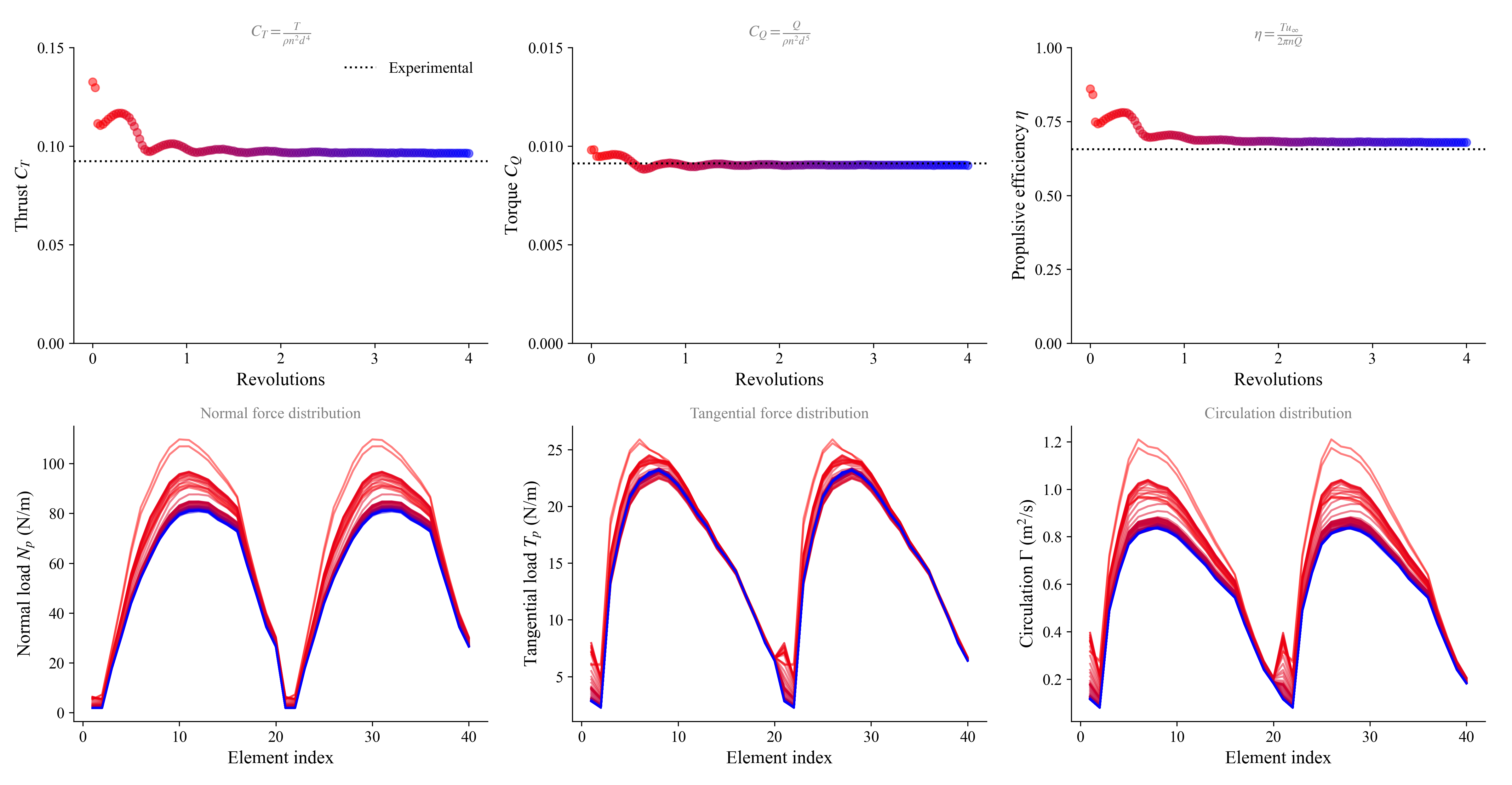
As the simulation runs, you will see the monitor shown below plotting the blade loading along with thrust and torque coefficients and propulsive efficiency.