Wing-on-Prop Interactions
In this example we show mount propellers on a swept wing. The wing is modeled using the actuator line model that represents the wing as a lifting line. This wing model is accurate for capturing wing-on-prop interactions. For instance, the rotor will experience an unsteady blade loading (and increased tonal noise) caused by the turning of the flow ahead of the wing leading edge. However, this simple wing model is not adecuate for capturing prop-on-wing interactions (see the next two sections to accurately predict prop-on-wing interactions).
#=##############################################################################
# DESCRIPTION
    Simulation of swept-back wing with twin props mounted mid span blowing on
    the wing.

# AUTHORSHIP
  * Author          : Eduardo J. Alvarez (edoalvarez.com)
  * Email           : Edo.AlvarezR@gmail.com
  * Created         : Apr 2023
  * Last updated    : Apr 2023
  * License         : MIT
=###############################################################################


import FLOWUnsteady as uns
import FLOWVLM as vlm
import FLOWVPM as vpm

run_name        = "blownwing-example"       # Name of this simulation
save_path       = run_name                  # Where to save this simulation
paraview        = true                      # Whether to visualize with Paraview

# ----------------- GEOMETRY PARAMETERS ----------------------------------------
# Wing geometry
b               = 2.489                     # (m) span length
ar              = 5.0                       # Aspect ratio b/c_tip
tr              = 1.0                       # Taper ratio c_tip/c_root
twist_root      = 0.0                       # (deg) twist at root
twist_tip       = 0.0                       # (deg) twist at tip
lambda          = 45.0                      # (deg) sweep
gamma           = 0.0                       # (deg) dihedral

# Rotor geometry
R               = 0.075*b                   # (m) rotor radius
Rhub            = 0.075*R                   # (m) hub radius
B               = 2                         # Number of blades
blade_file      = "apc10x7_blade.csv"       # Blade geometry
data_path       = uns.def_data_path         # Path to rotor database
pitch           = 5.0                       # (deg) collective pitch of blades
xfoil           = true                      # Whether to run XFOIL
ncrit           = 9                         # Turbulence criterion for XFOIL

# Vehicle assembly
AOAwing         = 4.2                       # (deg) wing angle of attack
spanpos         = [-0.5, 0.5]               # Semi-span position of each rotor, 2*y/b
xpos            = [-0.5, -0.5]              # x-position of rotors relative to LE, x/c
zpos            = [0.0, 0.0]                # z-position of rotors relative to LE, z/c
CWs             = [false, true]             # Clockwise rotation for each rotor
nrotors         = length(spanpos)           # Number of rotors

# Discretization
n_wing          = 50                        # Number of spanwise elements per side
r_wing          = 2.0                       # Geometric expansion of elements
n_rotor         = 15                        # Number of blade elements per blade
r_rotor         = 1/10                      # Geometric expansion of elements

# Check that we declared all the inputs that we need for each rotor
@assert length(spanpos)==length(xpos)==length(zpos)==length(CWs) ""*
    "Invalid rotor inputs! Check that spanpos, xpos, zpos, and CWs have the same length"

# ----------------- SIMULATION PARAMETERS --------------------------------------
# Vehicle motion
magVvehicle     = 49.7                      # (m/s) vehicle velocity
AOA             = 0.0                       # (deg) vehicle angle of attack

# Freestream
magVinf         = 1e-8                      # (m/s) freestream velocity
rho             = 0.93                      # (kg/m^3) air density
mu              = 1.85508e-5                # (kg/ms) air dynamic viscosity
speedofsound    = 342.35                    # (m/s) speed of sound
magVref         = sqrt(magVinf^2 + magVvehicle^2) # (m/s) reference velocity
qinf            = 0.5*rho*magVref^2         # (Pa) reference static pressure

Vinf(X, t)      = t==0 ? magVvehicle*[1,0,0] : magVinf*[1,0,0] # Freestream function

# Rotor operation
J               = 0.9                       # Advance ratio Vref/(nD)
RPM             = 60*magVref/(J*2*R)        # RPM

Rec             = rho * magVref * (b/ar) / mu       # Chord-based wing Reynolds number
ReD             = 2*pi*RPM/60*R * rho/mu * 2*R      # Diameter-based rotor Reynolds number
Matip           = 2*pi*RPM/60 * R / speedofsound    # Tip Mach number

println("""
    Vref:   $(round(magVref, digits=1)) m/s
    RPM:    $(RPM)
    Matip:  $(round(Matip, digits=3))
    ReD:    $(round(ReD, digits=0))
    Rec:    $(round(Rec, digits=0))
""")

# ----------------- SOLVER PARAMETERS ------------------------------------------

# Aerodynamic solver
VehicleType     = uns.UVLMVehicle           # Unsteady solver
# VehicleType     = uns.QVLMVehicle         # Quasi-steady solver
const_solution  = VehicleType==uns.QVLMVehicle  # Whether to assume that the
                                                # solution is constant or not
# Time parameters
nrevs           = 15                        # Number of revolutions in simulation
nsteps_per_rev  = 36                        # Time steps per revolution
nsteps          = const_solution ? 2 : nrevs*nsteps_per_rev # Number of time steps
ttot            = nsteps/nsteps_per_rev / (RPM/60)       # (s) total simulation time

# VPM particle shedding
p_per_step      = 4                         # Sheds per time step
shed_starting   = true                      # Whether to shed starting vortex
shed_unsteady   = true                      # Whether to shed vorticity from unsteady loading
unsteady_shedcrit = 0.001                   # Shed unsteady loading whenever circulation
                                            #  fluctuates by more than this ratio
max_particles   = nrotors*((2*n_rotor+1)*B)*nsteps*p_per_step + 1 # Maximum number of particles
max_particles   += (nsteps+1)*(2*n_wing*(p_per_step+1) + p_per_step)

# Regularization
sigma_vlm_surf  = b/100                     # VLM-on-VPM smoothing radius
sigma_rotor_surf= R/50                      # Rotor-on-VPM smoothing radius
lambda_vpm      = 2.125                     # VPM core overlap
                                            # VPM smoothing radius
sigma_vpm_overwrite = lambda_vpm * 2*pi*R/(nsteps_per_rev*p_per_step)
sigmafactor_vpmonvlm= 1                     # Shrink particles by this factor when
                                            #  calculating VPM-on-VLM/Rotor induced velocities

# Rotor solver
vlm_rlx         = 0.5                       # VLM relaxation <-- this also applied to rotors
hubtiploss_correction = vlm.hubtiploss_nocorrection # Hub and tip correction

# VPM solver
vpm_integration = vpm.rungekutta3           # VPM temporal integration scheme
# vpm_integration = vpm.euler

vpm_viscous     = vpm.Inviscid()            # VPM viscous diffusion scheme
# vpm_viscous   = vpm.CoreSpreading(-1, -1, vpm.zeta_fmm; beta=100.0, itmax=20, tol=1e-1)

vpm_SFS         = vpm.SFS_none              # VPM LES subfilter-scale model
# vpm_SFS       = vpm.DynamicSFS(vpm.Estr_fmm, vpm.pseudo3level_positive;
#                                   alpha=0.999, maxC=1.0,
#                                   clippings=[vpm.clipping_backscatter])

if VehicleType == uns.QVLMVehicle
    # Mute warnings regarding potential colinear vortex filaments. This is
    # needed since the quasi-steady solver will probe induced velocities at the
    # lifting line of the blade
    uns.vlm.VLMSolver._mute_warning(true)
end

println("""
    Resolving wake for $(round(ttot*magVref/b, digits=1)) span distances
""")

# ----------------- 1) VEHICLE DEFINITION --------------------------------------

# -------- Generate components
println("Generating geometry...")

# Generate wing
wing = vlm.simpleWing(b, ar, tr, twist_root, lambda, gamma;
                                    twist_tip=twist_tip, n=n_wing, r=r_wing);

# Pitch wing to its angle of attack
O = [0.0, 0.0, 0.0]                                 # New position
Oaxis = uns.gt.rotation_matrix2(0, -AOAwing, 0)     # New orientation
vlm.setcoordsystem(wing, O, Oaxis)

# Generate rotors
rotors = vlm.Rotor[]
for ri in 1:nrotors

    # Generate rotor
    rotor = uns.generate_rotor(R, Rhub, B, blade_file;
                                        pitch=pitch,
                                        n=n_rotor, CW=CWs[ri], blade_r=r_rotor,
                                        altReD=[RPM, J, mu/rho],
                                        xfoil=xfoil,
                                        ncrit=ncrit,
                                        data_path=data_path,
                                        verbose=true,
                                        verbose_xfoil=false,
                                        plot_disc=false
                                        );

    # Determine position along wing LE
    y = spanpos[ri]*b/2
    x = abs(y)*tand(lambda) + xpos[ri]*b/ar
    z = abs(y)*tand(gamma) + zpos[ri]*b/ar

    # Account for angle of attack of wing
    nrm = sqrt(x^2 + z^2)
    x = (x==0 ? 1 : sign(x))*nrm*cosd(AOAwing)
    z = -(z==0 ? 1 : sign(z))*nrm*sind(AOAwing)

    # Translate rotor to its position along wing
    O = [x, y, z]                                       # New position
    Oaxis = uns.gt.rotation_matrix2(0, 0, 180)          # New orientation
    vlm.setcoordsystem(rotor, O, Oaxis)

    push!(rotors, rotor)
end


# -------- Generate vehicle
println("Generating vehicle...")

# System of all FLOWVLM objects
system = vlm.WingSystem()

vlm.addwing(system, "Wing", wing)

for (ri, rotor) in enumerate(rotors)
    vlm.addwing(system, "Rotor$(ri)", rotor)
end

# System solved through VLM solver
vlm_system = vlm.WingSystem()
vlm.addwing(vlm_system, "Wing", wing)

# Systems of rotors
rotor_systems = (rotors, );

# System that will shed a VPM wake
wake_system = vlm.WingSystem()              # System that will shed a VPM wake
vlm.addwing(wake_system, "Wing", wing)
                                            # NOTE: Do NOT include rotor when using the quasi-steady solver
if VehicleType != uns.QVLMVehicle
    for (ri, rotor) in enumerate(rotors)
        vlm.addwing(wake_system, "Rotor$(ri)", rotor)
    end
end

# Pitch vehicle to its angle of attack
O = [0.0, 0.0, 0.0]                                 # New position
Oaxis = uns.gt.rotation_matrix2(0, -AOA, 0)         # New orientation
vlm.setcoordsystem(system, O, Oaxis)

vehicle = VehicleType(   system;
                            vlm_system=vlm_system,
                            rotor_systems=rotor_systems,
                            wake_system=wake_system
                         );


# ------------- 2) MANEUVER DEFINITION -----------------------------------------
# Non-dimensional translational velocity of vehicle over time
Vvehicle(t) = [-1, 0, 0]        # <---- Vehicle is traveling in the -x direction

# Angle of the vehicle over time
anglevehicle(t) = zeros(3)

# RPM control input over time (RPM over `RPMref`)
RPMcontrol(t) = 1.0

angles = ()                                 # Angle of each tilting system (none)
RPMs = (RPMcontrol, )                       # RPM of each rotor system

maneuver = uns.KinematicManeuver(angles, RPMs, Vvehicle, anglevehicle)


# ------------- 3) SIMULATION DEFINITION ---------------------------------------

Vref = magVvehicle                          # Reference velocity to scale maneuver by
RPMref = RPM                                # Reference RPM to scale maneuver by
Vinit = Vref*Vvehicle(0)                    # Initial vehicle velocity
Winit = pi/180*(anglevehicle(1e-6) - anglevehicle(0))/(1e-6*ttot)  # Initial angular velocity

simulation = uns.Simulation(vehicle, maneuver, Vref, RPMref, ttot;
                                                    Vinit=Vinit, Winit=Winit);

# ------------- 4) MONITORS DEFINITIONS ----------------------------------------

# Generate function that computes wing aerodynamic forces
calc_aerodynamicforce_fun = uns.generate_calc_aerodynamicforce(;
                                    add_parasiticdrag=true,
                                    add_skinfriction=true,
                                    airfoilpolar="xf-rae101-il-1000000.csv"
                                    )

L_dir(t) = [0, 0, 1]                        # Direction of lift
D_dir(t) = [1, 0, 0]                        # Direction of drag

# Generate wing monitor
monitor_wing = uns.generate_monitor_wing(wing, Vinf, b, ar,
                                            rho, qinf, nsteps;
                                            calc_aerodynamicforce_fun=calc_aerodynamicforce_fun,
                                            L_dir=L_dir,
                                            D_dir=D_dir,
                                            save_path=save_path,
                                            run_name=run_name*"-wing",
                                            figname="wing monitor",
                                            )

# Generate rotors monitor
monitor_rotors = uns.generate_monitor_rotors(rotors, J, rho, RPM, nsteps;
                                            t_scale=RPM/60,        # Scaling factor for time in plots
                                            t_lbl="Revolutions",   # Label for time axis
                                            save_path=save_path,
                                            run_name=run_name*"-rotors",
                                            figname="rotors monitor",
                                            )
# Concatenate monitors
monitors = uns.concatenate(monitor_wing, monitor_rotors)


# ------------- 5) RUN SIMULATION ----------------------------------------------
println("Running simulation...")


# Run simulation
uns.run_simulation(simulation, nsteps;
                    # ----- SIMULATION OPTIONS -------------
                    Vinf=Vinf,
                    rho=rho, mu=mu, sound_spd=speedofsound,
                    # ----- SOLVERS OPTIONS ----------------
                    p_per_step=p_per_step,
                    max_particles=max_particles,
                    vpm_integration=vpm_integration,
                    vpm_viscous=vpm_viscous,
                    vpm_SFS=vpm_SFS,
                    sigma_vlm_surf=sigma_vlm_surf,
                    sigma_rotor_surf=sigma_rotor_surf,
                    sigma_vpm_overwrite=sigma_vpm_overwrite,
                    sigmafactor_vpmonvlm=sigmafactor_vpmonvlm,
                    vlm_rlx=vlm_rlx,
                    hubtiploss_correction=hubtiploss_correction,
                    shed_starting=shed_starting,
                    shed_unsteady=shed_unsteady,
                    unsteady_shedcrit=unsteady_shedcrit,
                    extra_runtime_function=monitors,
                    # ----- OUTPUT OPTIONS ------------------
                    save_path=save_path,
                    run_name=run_name,
                    save_wopwopin=true,  # <--- Generates input files for PSU-WOPWOP noise analysis
                    );


# ----------------- 6) VISUALIZATION -------------------------------------------
if paraview
    println("Calling Paraview...")

    # Files to open in Paraview
    files = joinpath(save_path, run_name*"_pfield...xmf;")
    for ri in 1:nrotors
        for bi in 1:B
            global files *= run_name*"_Rotor$(ri)_Blade$(bi)_loft...vtk;"
        end
    end
    files *= run_name*"_Wing_vlm...vtk;"

    # Call Paraview
    run(`paraview --data=$(files)`)

end
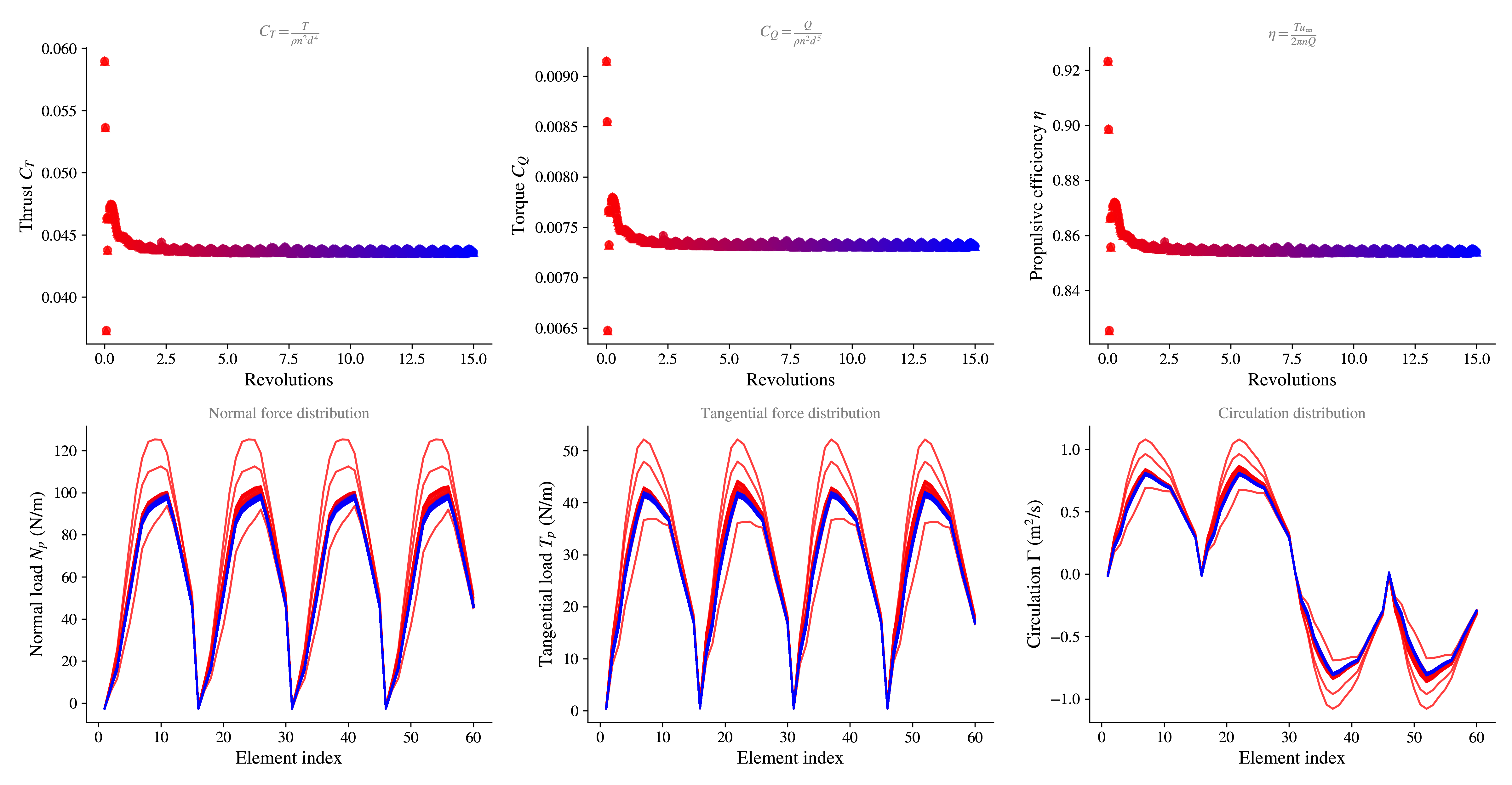
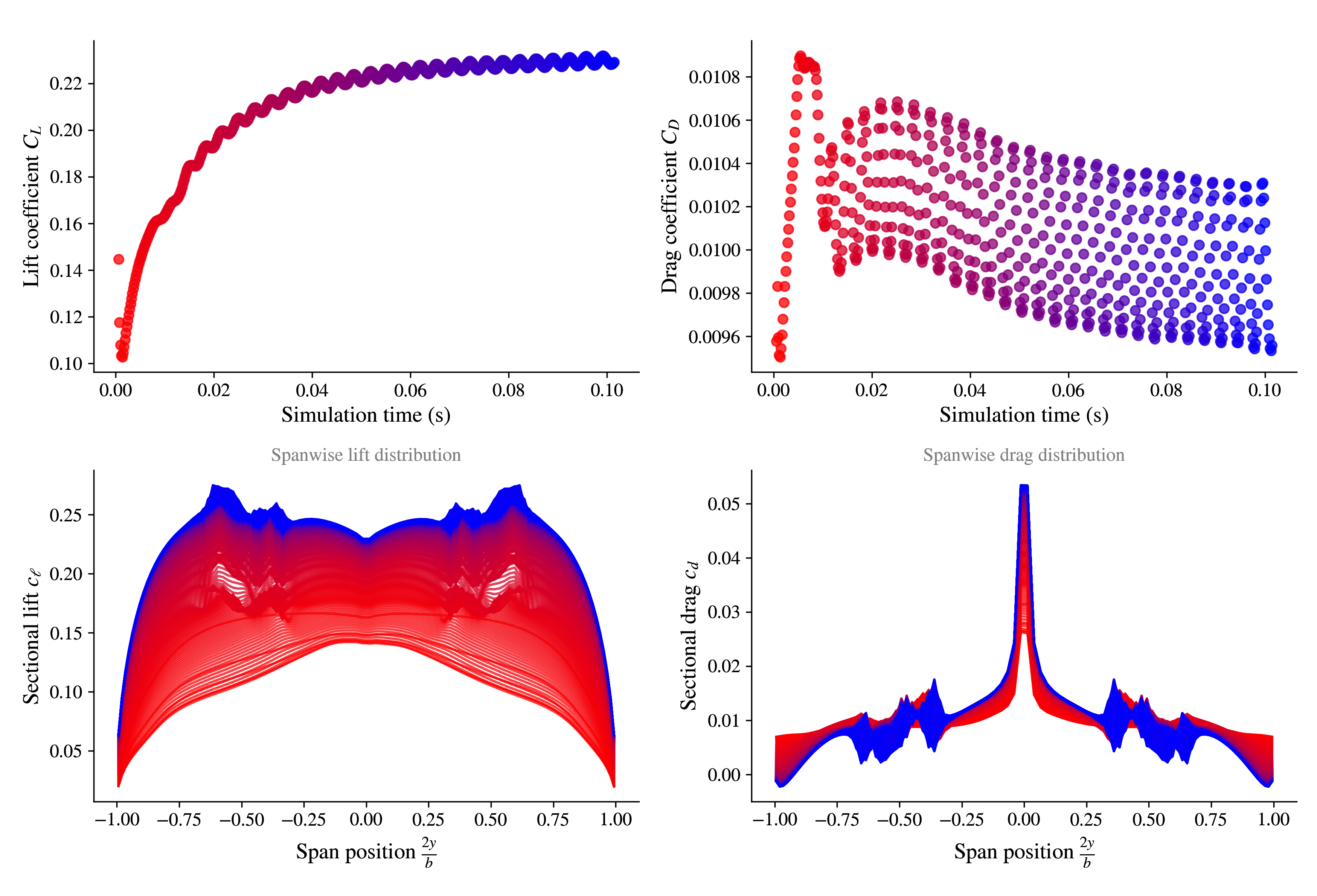
(red = beginning, blue = end)
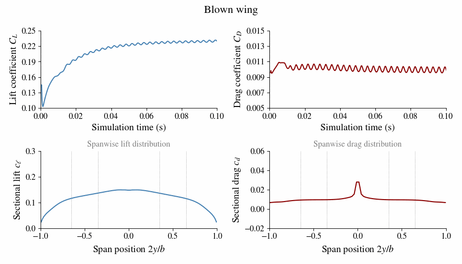
Check the full example under examples/blownwing/ to see how to postprocess the simulation and generate this animation.