Surface of Revolution Method

Following the concept of bodies of revolution where a contour is revolved around an axis, this method generates the surface of such revolution.

Node and Cell Indexing

Standard input:

• Contour drawn in the $+y$ quadrants following the Selig airfoil format (starting at the trailing edge, progressing to the leading edge along the upper surface, and returning to the trailing edge along the lower surface).
• The contour can be a closed curve describing the a toroidal cross section (as in the case of the duct), or an open contour along the $y=0$ axis describing the half surface of a cylindrical body of revolution (as in the case of the centerbody).

Following these guidelines, GeometricTools.surface_revolution returns a revolved quadrilateral surface with the following node and cell indexing pattern:

First Coordinate	Second Coordinate

Node Index	Cell Index

Cell (1, 1)	Cell (40, 1)	Cell (39, 2)

OBSERVATION: The following examples show how to use the revolution method directly from the GeometricTools package. In order to use this grid in the definition of a body, the quadrilateral panels must by transformed into triangular panels through GeometricTools.GridTriangleSurface(orggrid, dimsplit).

Example — Rotor hub

First, we need a profile to revolve consisting of a collection of points. This can be predefined and read as a csv file (for example), or defined programmatically. Here we show how to define the contour programmatically:

import PyPlot as plt

Rhub = 0.375 * 0.02542        # (m) radius of hub
Rinn = Rhub / 2               # (m) inner hole radius
Rsec1 = Rinn                # (m) radius of first hole
Rsec2 = 3 / 1000              # (m) radius of second hole
Thub = Rhub                 # (m) thickness of hub
dsec1 = 3 / 1000              # (m) depth of first hole

Rfillet = 2 / 1000            # (m) Fillet radius
Nfillet = 30                # Points along fillet
Cfillet = [Rhub, Thub] .- Rfillet      # Center of fillet

points_fillet = [Cfillet .+ Rfillet * [sin(a), cos(a)]
                        for a in range(0, stop=pi/2, length=Nfillet)]

points = hcat(
              [Rsec2, Thub-dsec1],
              [Rsec1, Thub-dsec1],
              [Rsec1, Thub],
              points_fillet...,
              [Rhub, 0],
              [Rsec1, 0],
              [Rsec1, dsec1],
              [Rsec2, dsec1],
              [Rsec2, Thub-dsec1]
             )'

x = [points[i,1] for i in 1:size(points,1)]
y = [points[i,2] for i in 1:size(points,1)]

plt.figure(figsize=[5,5]*2/3)
plt.plot(x,y, "--ok")
plt.plot([Cfillet[1]], [Cfillet[2]], "xr")
plt.xlim([0, Rhub*1.25])
plt.ylim([-Rhub*0.125, Rhub*1.125]);

plt.savefig(joinpath(img_path, "geometry-hubcontour00.png"), transparent=true, dpi=300)

import FLOWPanel as pnl

save_path = "./"
file_name = "hub00"

thetaNDIVS = 180          # Number of angular sections
loop_dim = 1             # Loops the parametric grid

# Creates body of revolution
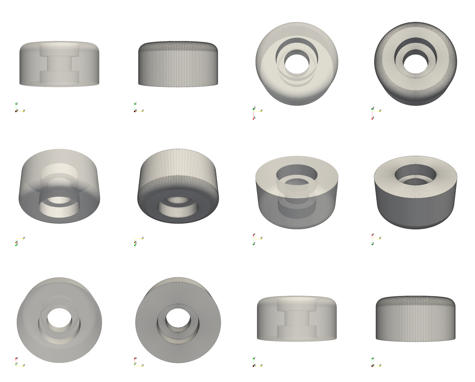
grid = pnl.gt.surface_revolution(points, thetaNDIVS; loop_dim=loop_dim)

# Save vtk and call paraview
pnl.gt.save(grid, file_name; path=save_path, format="vtk")

run(`paraview --data=$(joinpath(save_path, file_name)).vtk`)

Example — Tilted revolution

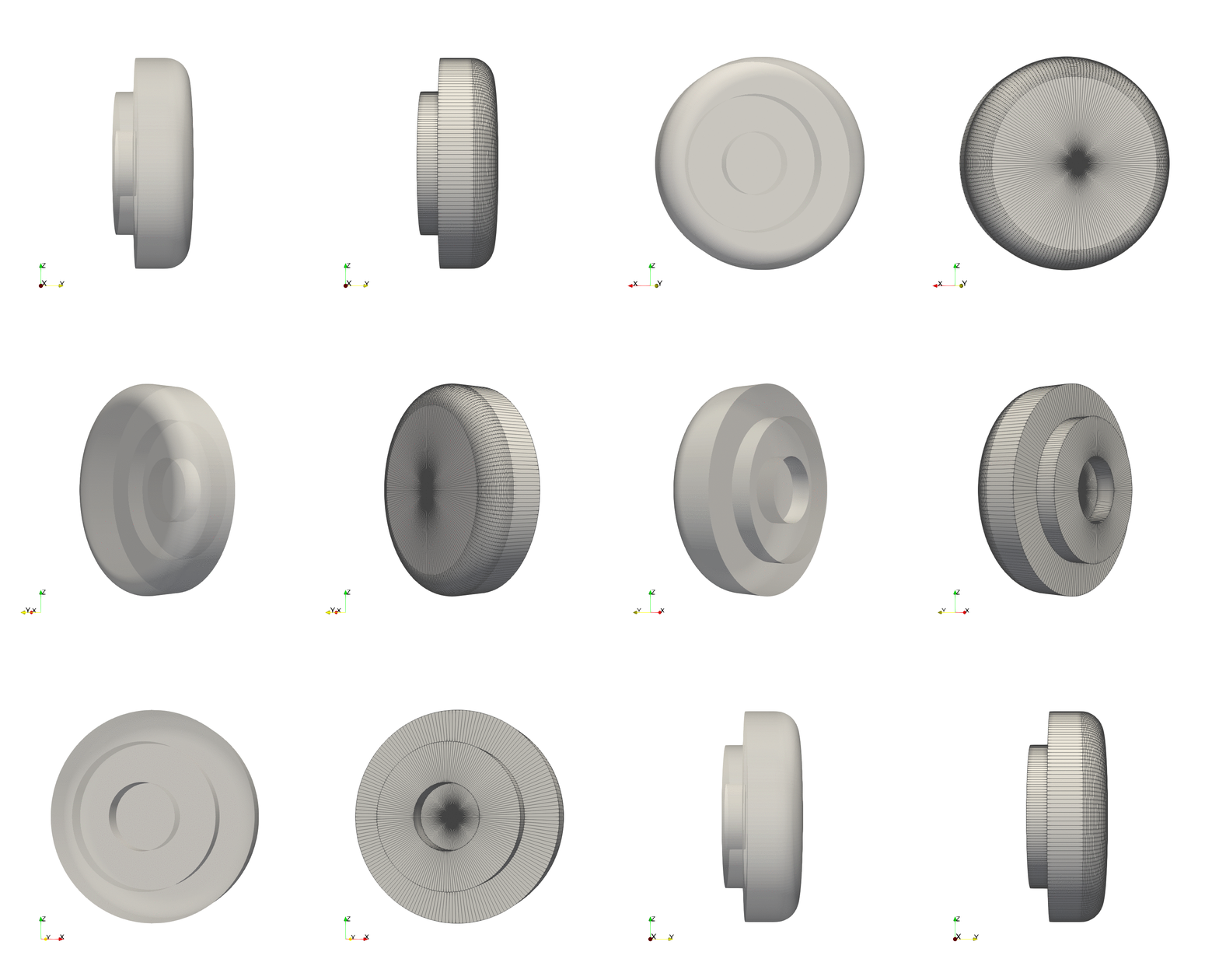
By using the optional argument axis_angle we can tilt the angle about which to do the revolution. To exemplify this, using the previous contour we will tilting the axis by $90^\circ$ about the $z$-axis, resulting in a revolution about the $y$-axis:

axis_angle = 90          # Axis tilting

grid = pnl.gt.surface_revolution(points, thetaNDIVS;
                                    loop_dim=loop_dim,
                                    axis_angle=axis_angle)

# Save vtk and call paraview
pnl.gt.save(grid, file_name; path=save_path, format="vtk")

run(`paraview --data=$(joinpath(save_path, file_name)).vtk`)

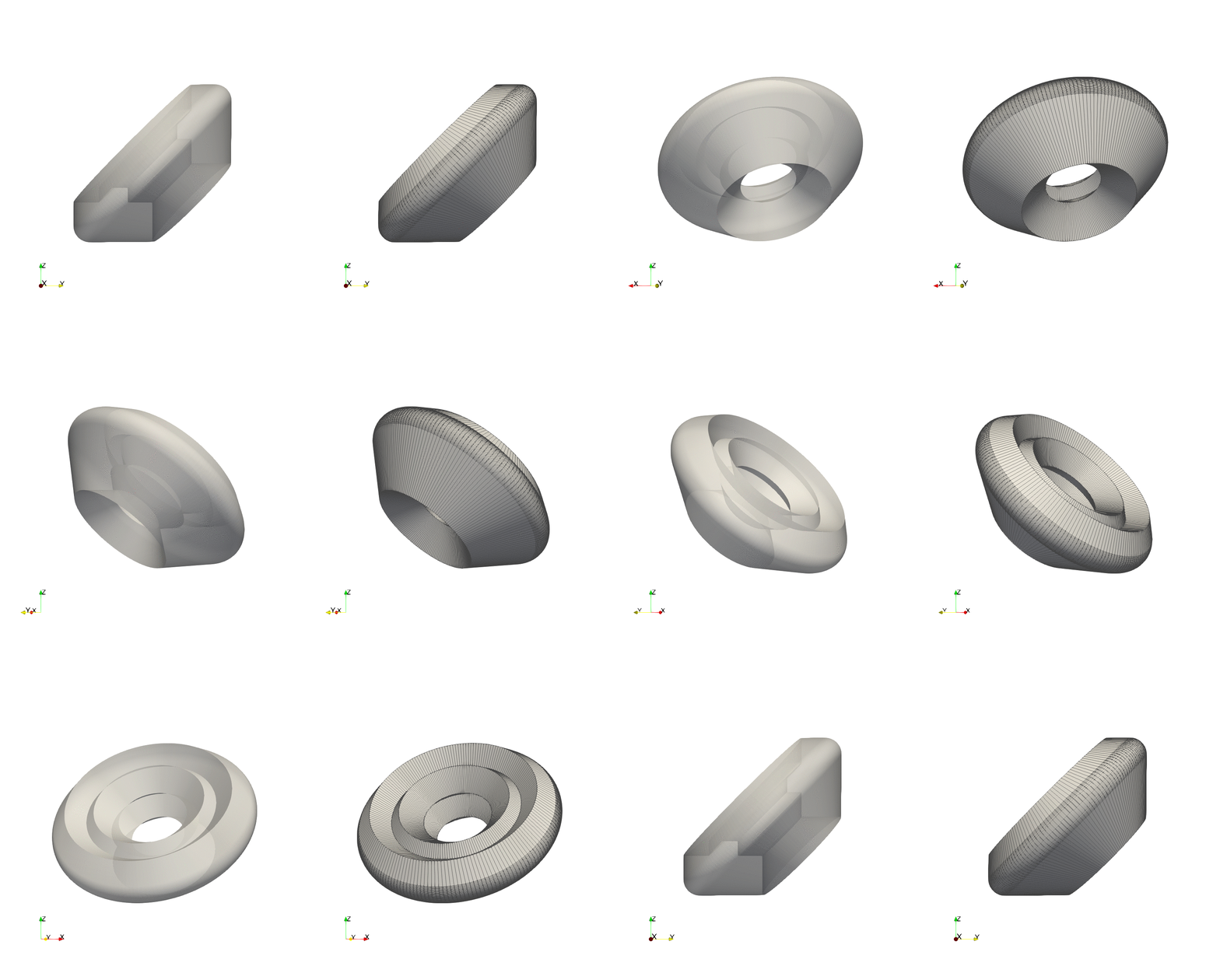
And here is what we get by tilting the axis by $45^\circ$ about the $z$-axis:

axis_angle = 45          # Axis tilting

grid = pnl.gt.surface_revolution(points, thetaNDIVS;
                                    loop_dim=loop_dim,
                                    axis_angle=axis_angle)

# Save vtk and call paraview
pnl.gt.save(grid, file_name; path=save_path, format="vtk")

run(`paraview --data=$(joinpath(save_path, file_name)).vtk`)

Example — Incomplete revolution

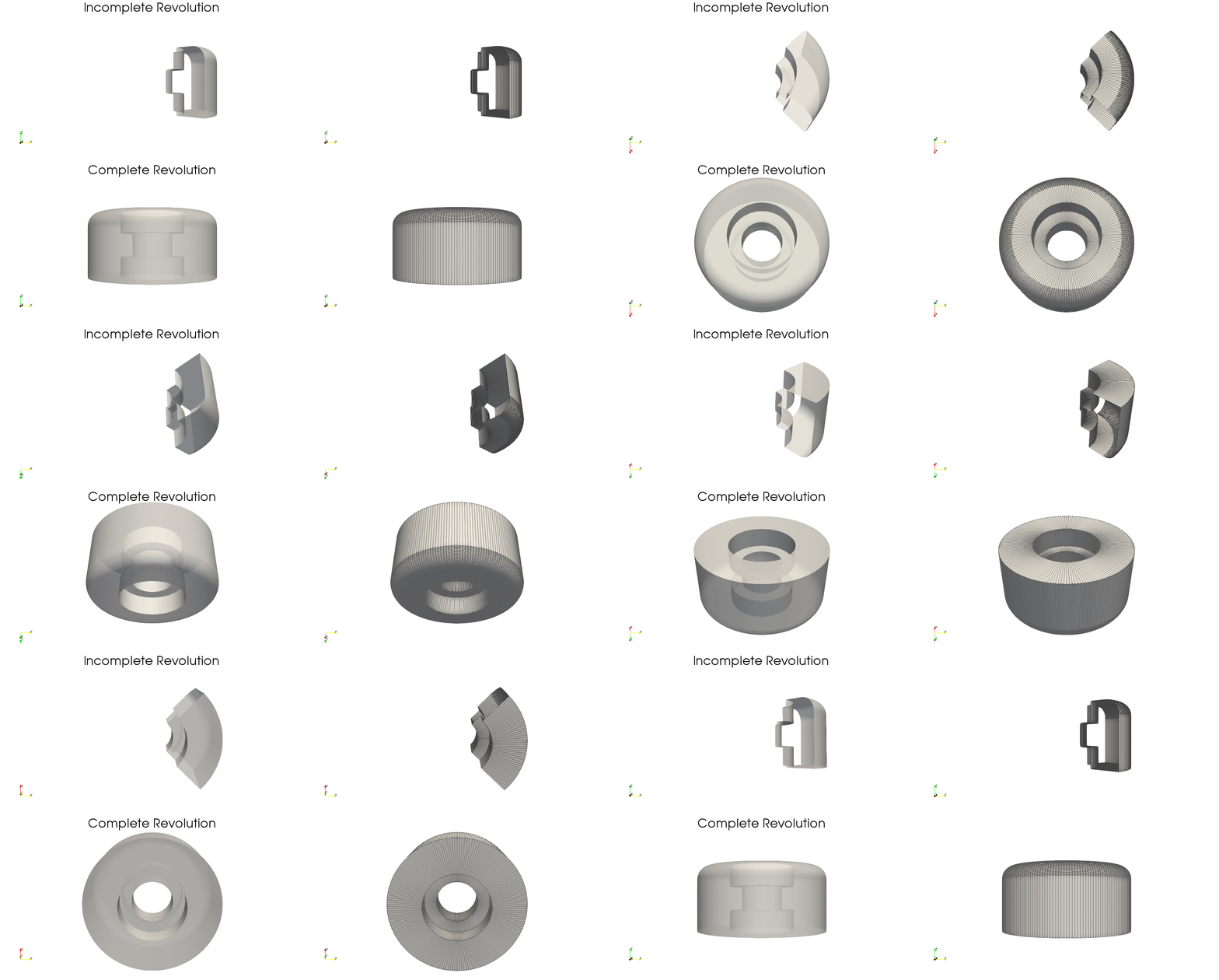
Using the arguments low_a and up_a we can set the lower and upper bound angles of the revolution to create an incomplete body of revolution:

thetaNDIVS = 45          # Number of angular sections
loop_dim = 1             # Loops the parametric grid
low_a = -45              # Lower bound of revolution angle
up_a = 45                # Upper bound of revolution angle

grid = pnl.gt.surface_revolution(points, thetaNDIVS;
                                    loop_dim=loop_dim,
                                    low_a=low_a, up_a=up_a)

# Save vtk and call paraview
pnl.gt.save(grid, file_name; path=save_path, format="vtk")

run(`paraview --data=$(joinpath(save_path, file_name)).vtk`)