Import Mesh and Solve
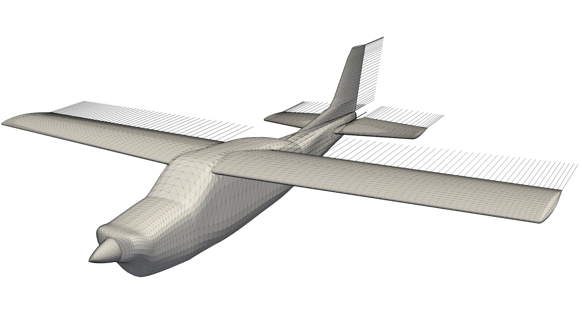
Here we import the mesh into FLOWPanel using Meshes.jl, identify the trailing edge, and run the watertight solver.
We have pre-generated and uploaded an OpenVSP mesh to this example so that you can run this section without needing to complete the previous sections. However, if you would like to use your own mesh, simply change read_path, meshfile, and trailingedges to point to your files.
#=##############################################################################
# DESCRIPTION
Cessna 210 aircraft. The mesh used in this analysis was created using
OpenVSP.
# AUTHORSHIP
* Author : Eduardo J. Alvarez
* Email : Edo.AlvarezR@gmail.com
* Created : Apri 2024
* License : MIT License
=###############################################################################
import FLOWPanel as pnl
import FLOWPanel: norm, dot, cross
import Meshes
import GeoIO
import Rotations: RotX, RotY, RotZ
run_name = "cessna" # Name of this run
save_path = run_name # Where to save outputs
paraview = true # Whether to visualize with Paraview
read_path = joinpath(pnl.examples_path, "data") # Where to read Gmsh files from
# ----------------- SIMULATION PARAMETERS --------------------------------------
AOA = 4.0 # (deg) freestream angle of attack
magVinf = 180 * 0.514444 # (m/s) freestream velocity
rho = 0.71461 # (kg/m^3) air density at 17300 ft
# ----------------- GEOMETRY DESCRIPTION ---------------------------------------
meshfile = "cessna.msh" # Gmsh file to read
offset = [0, 0, 0] # Offset to center the mesh
rotation = RotX(0*pi/180) * RotY(0*pi/180) * RotX(0*pi/180) # Rotation to align mesh
scaling = 0.3048 # Factor to scale mesh dimensions (ft -> m)
trailingedges = [ # Gmsh files with trailing edges
# ( Gmsh file, span sorting function, junction criterion, closed )
( "cessna-TE-leftwing.msh", X -> dot(X, [0, 1, 0]), X -> abs(X[2]) - 0.67, false ),
( "cessna-TE-rightwing.msh", X -> dot(X, [0, 1, 0]), X -> abs(X[2]) - 0.67, false ),
( "cessna-TE-leftelevator.msh", X -> dot(X, [0, 1, 0]), X -> abs(X[2]) - 0.23, false ),
( "cessna-TE-rightelevator.msh", X -> dot(X, [0, 1, 0]), X -> abs(X[2]) - 0.23, false ),
( "cessna-TE-rudder.msh", X -> dot(X, [0, 0, 1]), X -> X[3] - 0.65, false ),
]
flip = true # Whether to flip control points against the direction of normals
# NOTE: use `flip=true` if the normals
# point inside the body
bref = 11.2014 # (m) reference span
cref = 1.449324 # (m) reference chord
Sref = 16.2344 # (m^2) reference area
Xac = [2.815, 0, 0.4142] # (m) aerodynamic center for
# calculation of moments
# Define function used for reading Gmsh files
meshreader(file) = GeoIO.load(file).geometry
# Format input for `generate_multibody(...)`
meshfiles = [ ("Airframe", meshfile, flip) ]
# ----------------- SOLVER SETTINGS -------------------------------------------
# Solver: direct linear solver for open bodies
# bodytype = pnl.RigidWakeBody{pnl.VortexRing} # Wake model and element type
# Solver: least-squares solver for watertight bodies
bodytype = pnl.RigidWakeBody{pnl.VortexRing, 2}
# ----------------- GENERATE BODY ----------------------------------------------
body, elsprescribe = pnl.generate_multibody(bodytype, meshfiles, trailingedges, meshreader;
tolerance=0.001,
lengthscale=bref,
read_path=read_path,
offset=offset, rotation=rotation, scaling=scaling,
)
# ----------------- CALL SOLVER ------------------------------------------------
println("Solving body...")
# Freestream vector
Vinf = magVinf*[cos(AOA*pi/180), 0, sin(AOA*pi/180)]
# Freestream at every control point
Uinfs = repeat(Vinf, 1, body.ncells)
# Unitary direction of semi-infinite vortex at points `a` and `b` of each
# trailing edge panel
Das = repeat(Vinf/magVinf, 1, body.nsheddings)
Dbs = repeat(Vinf/magVinf, 1, body.nsheddings)
# Solve body (panel strengths) giving `Uinfs` as boundary conditions and
# `Das` and `Dbs` as trailing edge rigid wake direction
@time pnl.solve(body, Uinfs, Das, Dbs; elprescribe=elsprescribe)
# ----------------- POST PROCESSING ----------------------------------------
println("Post processing...")
# Calculate surface velocity U on the body
Us = pnl.calcfield_U(body, body)
# NOTE: Since the boundary integral equation of the potential flow has a
# discontinuity at the boundary, we need to add the gradient of the
# doublet strength to get an accurate surface velocity
# Calculate surface velocity U_∇μ due to the gradient of the doublet strength
UDeltaGamma = pnl.calcfield_Ugradmu(body)
# UDeltaGamma = pnl.calcfield_Ugradmu(body; sharpTE=true, force_cellTE=false)
# Save this intermediate result in a separate field for debugging
pnl.add_field(body, "Uinfind", "vector", collect.(eachcol(Us)), "cell")
# Add both velocities together
pnl.addfields(body, "Ugradmu", "U")
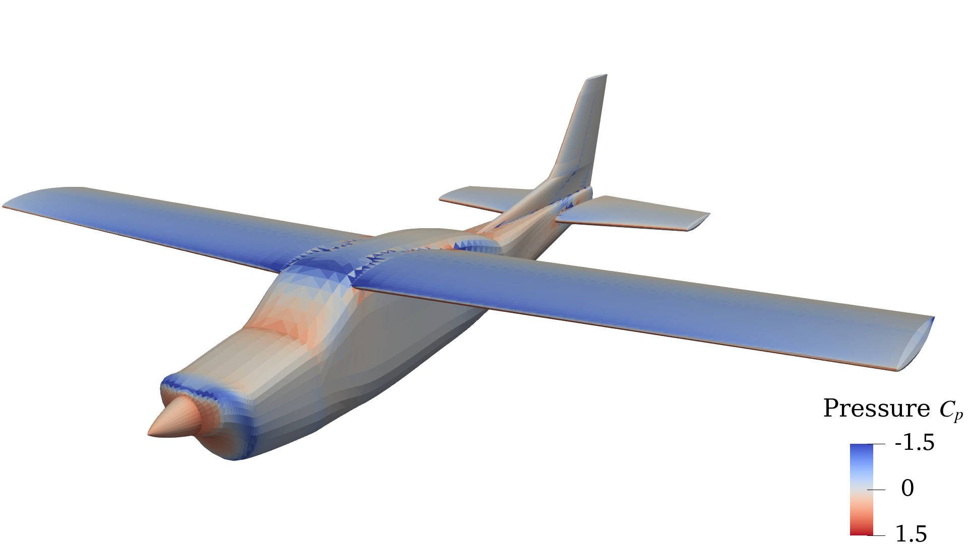
# Calculate pressure coefficient (based on U + U_∇μ)
@time Cps = pnl.calcfield_Cp(body, magVinf)
# Calculate the force of each panel (based on Cp)
@time Fs = pnl.calcfield_F(body, magVinf, rho)
# Calculate total force of the vehicle decomposed as lift, drag, and sideslip
Dhat = Vinf/norm(Vinf) # Drag direction
Shat = [0, 1, 0] # Span direction
Lhat = cross(Dhat, Shat) # Lift direction
LDS = pnl.calcfield_LDS(body, Lhat, Dhat)
L, D, S = collect(eachcol(LDS))
# Force coefficients
nondim = 0.5*rho*magVinf^2*Sref # Normalization factor
CL = sign(dot(L, Lhat)) * norm(L) / nondim
CD = sign(dot(D, Dhat)) * norm(D) / nondim
# Integrated moment decomposed into rolling, pitching, and yawing moments
lhat = Dhat # Rolling direction
mhat = Shat # Pitching direction
nhat = Lhat # Yawing direction
lmn = pnl.calcfield_lmn(body, Xac, lhat, mhat, nhat)
roll, pitch, yaw = collect(eachcol(lmn))
# Moment coefficients
nondim = 0.5*rho*magVinf^2*Sref*cref # Normalization factor
Cl = sign(dot(roll, lhat)) * norm(roll) / nondim
Cm = sign(dot(pitch, mhat)) * norm(pitch) / nondim
Cn = sign(dot(yaw, nhat)) * norm(yaw) / nondim
@show L
@show D
@show CL
@show CD
@show Cl
@show Cm
@show Cn
# ----------------- VISUALIZATION ------------------------------------------
# Save body as VTK
vtks = save_path*"/" # String with VTK output files
vtks *= pnl.save(body, run_name; path=save_path, debug=false)
# NOTE: using `debug=true` outputs the control points and normal, but it takes
# much longer since it also calculates the velocity at those points
# Call Paraview
if paraview
run(`paraview --data=$(vtks)`)
endRun time: ~100 seconds on a Dell Precision 7760 laptop (no GPU).
| VSPAERO | FLOWPanel | |
|---|---|---|
| Lift $C_L$ | 0.499 | 0.554 |
| Drag $C_D$ | 0.0397 | 0.0496 |

You can also automatically run this example with the following command:
import FLOWPanel as pnl

include(joinpath(pnl.examples_path, "cessna.jl"))- Check whether normals point into the body: Using the flag
debug=trueinpnl.save(body, run_name; path=save_path, debug=true)will output the control points of the body along with the associated normal vector of each panel. We recommend opening the body and control points in ParaView and visualizing the normals with the Glyph filter. Whenever the normals are pointing into the body, the user needs to flip the offset of the control points withCPoffset=-1e-14or any other negligibly small negative number. This won't flip the normals outwards, but it will flip the zero-potential domain from outwards back to inside the body (achieved by shifting the control points slightly into the body). If you pull up the solution in ParaView and realize that the surface velocity is much smaller than the freestream everywhere along the aircraft, that's an indication that the normals are point inwards and you need to setCPoffsetto be negative. - Check that the trailing edge was correctly identified:
pnl.save(body, run_name; path=save_path)automatically outputes the wake. We recommend opening the body and wake in ParaView and visually inspecting that the wake runs along the trailing edge line that you defined undertrailingedge. If not successful, increase the resolution oftrailingedgeand tighten the tolerance to something small likepnl.calc_shedding(grid, trailingedge; tolerance=0.0001*span). - Choose the right solver for the geometry: Use the least-squares solver with watertight bodies (
bodytype = pnl.RigidWakeBody{pnl.VortexRing, 2}), and the direct linear solver with open bodies (bodytype = pnl.RigidWakeBody{pnl.VortexRing}). The least-squares solver runs much faster in GPU (pnl.solve(body, Uinfs, Das, Dbs; GPUArray=CUDA.CuArray{Float32})), but it comes at the price of sacrificing accuracy (single precision numbers as opposed to double).
To help you practice in ParaView, we have uploaded the solution files of this simulation along with the ParaView state file (.pvsm) that we used to generate the visualizations shown above: DOWNLOAD
To open in ParaView: File → Load State → cessna.pvsm then select "Search files under specified directory" and point it to the folder with the outputs of FLOWPanel.