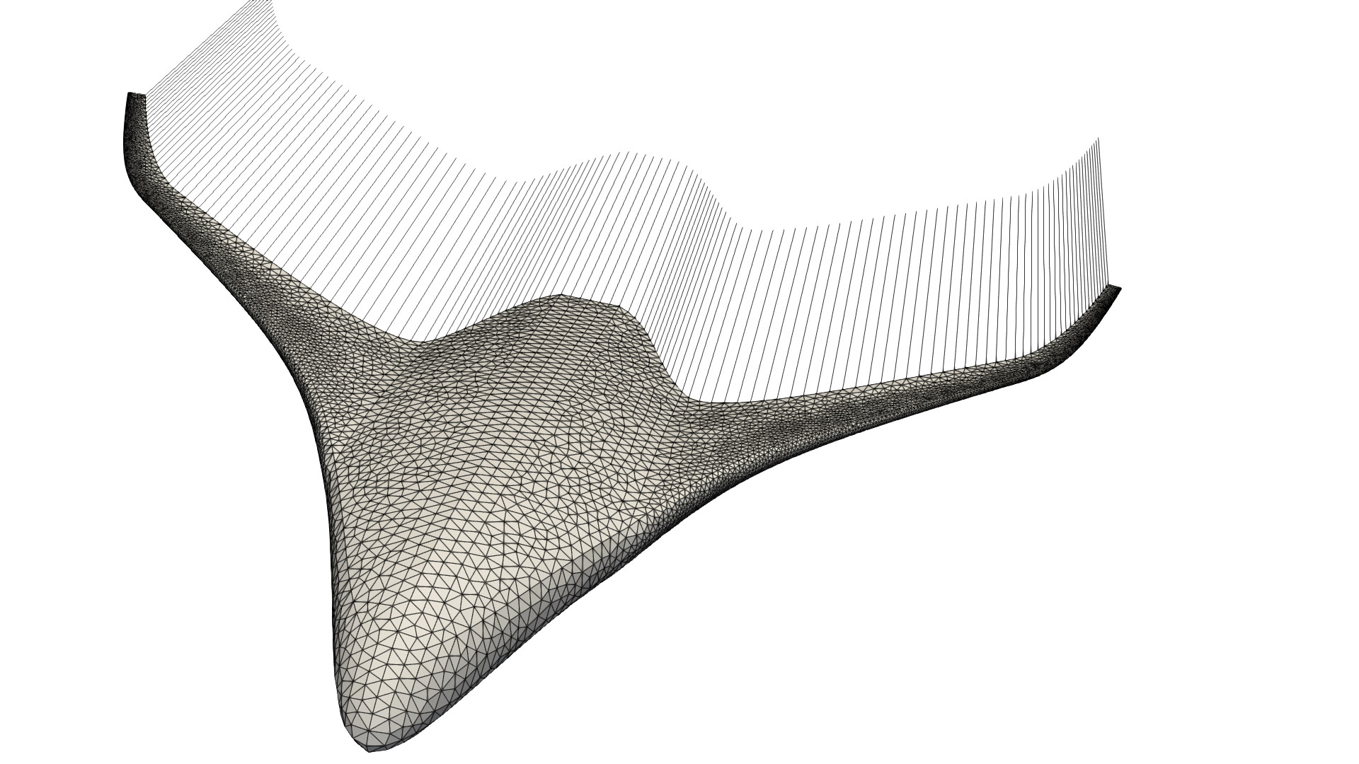
Import Mesh and Solve
Here we import the mesh into FLOWPanel using Meshes.jl, identify the trailing edge, and run the watertight solver.
We have pre-generated and uploaded a Gmsh mesh to this example so that you can run this section without needing to complete the previous sections. However, if you would like to use your own mesh, simply change read_path, meshfile, and trailingedgefile to point to your files.
#=##############################################################################
# DESCRIPTION
Blended wing body resembling the Airbus ZEROe BWB twin-engine subscale
model. The mesh used in this analysis was created using SolidWorks + Gmsh.
# AUTHORSHIP
* Author : Eduardo J. Alvarez
* Email : Edo.AlvarezR@gmail.com
* Created : April 2024
* License : MIT License
=###############################################################################
import FLOWPanel as pnl
import FLOWPanel: norm, dot, cross
import Meshes
import GeoIO
import Rotations: RotX, RotY, RotZ
# import CUDA # Uncomment this to use GPU (if available)
run_name = "blendedwing" # Name of this run
save_path = run_name # Where to save outputs
paraview = true # Whether to visualize with Paraview
read_path = joinpath(pnl.examples_path, "data") # Where to read Gmsh files from
# ----------------- SIMULATION PARAMETERS --------------------------------------
AOA = 10.0 # (deg) freestream angle of attack
magVinf = 30.0 # (m/s) freestream velocity
rho = 1.225 # (kg/m^3) air density
# ----------------- GEOMETRY DESCRIPTION ---------------------------------------
meshfile = joinpath(read_path, "zeroebwb.msh") # Gmsh file to read
trailingedgefile= joinpath(read_path, "zeroebwb-TE.msh") # Gmsh file with trailing edge
symcoordinate = 2 # Symmetric coordinate to reflect the body (`nothing` to omit)
offset = [0, 0, 0] # Offset to center the mesh
rotation = RotZ(-90*pi/180)*RotX(90*pi/180) # Rotation to align mesh
scaling = 2e-3 # Factor to scale original mesh to
# the approximate dimensions of the
# ZEROEe BWB subscale model
spandir = [0, 1, 0] # Span direction used to orient the trailing edge
flip = false # Whether to flip control points against the direction of normals
# NOTE: use `flip=true` if the normals
# point inside the body
Sref = 3.23^2 / 8.0 # (m^2) reference area
# ----------------- SOLVER SETTINGS -------------------------------------------
# Solver: direct linear solver for open bodies
# bodytype = pnl.RigidWakeBody{pnl.VortexRing} # Wake model and element type
# Solver: least-squares solver for watertight bodies
bodytype = pnl.RigidWakeBody{pnl.VortexRing, 2}
# Processing
clip_Cp = 1 - 342.0/magVinf # Clip pressure coefficients that are lower than this threshold
# ----------------- GENERATE BODY ----------------------------------------------
# Read Gmsh mesh
msh = GeoIO.load(meshfile)
msh = msh.geometry
# Read Gmsh line of trailing edge
TEmsh = GeoIO.load(trailingedgefile)
TEmsh = TEmsh.geometry
# Transform the original mesh: Translate, rotate, and scale
msh = msh |> Meshes.Translate(offset...) |> Meshes.Rotate(rotation) |> Meshes.Scale(scaling)
# Apply the same transformations to the trailing edge
TEmsh = TEmsh |> Meshes.Translate(offset...) |> Meshes.Rotate(rotation) |> Meshes.Scale(scaling)
# Mirror the original mesh to obtain a symmetric mesh of the airframe
if !isnothing(symcoordinate)
msh = pnl.gt.mirror(msh, symcoordinate)
end
# Uncomment this to do 10 smoothing iterations on the mesh
# msh = msh |> Meshes.TaubinSmoothing(10)
# Wrap Meshes object into a Grid object from GeometricTools
grid = pnl.gt.GridTriangleSurface(msh)
# Convert TE Meshes object into a matrix of points used to identify the trailing edge
trailingedge = pnl.gt.vertices2nodes(TEmsh.vertices)
# Sort TE points from left to right
trailingedge = sortslices(trailingedge; dims=2, by = X -> pnl.dot(X, spandir))
# Estimate span length (used as a reference length)
spantips = extrema(X -> pnl.dot(X, spandir), eachcol(trailingedge))
span = spantips[2] - spantips[1]
# Generate TE shedding matrix
shedding = pnl.calc_shedding(grid, trailingedge; tolerance=0.001*span)
# Generate paneled body
body = bodytype(grid, shedding; CPoffset=(-1)^flip * 1e-14)
println("Number of panels:\t$(body.ncells)")
# ----------------- CALL SOLVER ------------------------------------------------
println("Solving body...")
# Freestream vector
Vinf = magVinf*[cos(AOA*pi/180), 0, sin(AOA*pi/180)]
# Freestream at every control point
Uinfs = repeat(Vinf, 1, body.ncells)
# Unitary direction of semi-infinite vortex at points `a` and `b` of each
# trailing edge panel
Das = repeat(Vinf/magVinf, 1, body.nsheddings)
Dbs = repeat(Vinf/magVinf, 1, body.nsheddings)
# Solve body (panel strengths) giving `Uinfs` as boundary conditions and
# `Das` and `Dbs` as trailing edge rigid wake direction
@time pnl.solve(body, Uinfs, Das, Dbs)
# Uncomment this to use GPU instead (if available)
# @time pnl.solve(body, Uinfs, Das, Dbs; GPUArray=CUDA.CuArray{Float32})
# ----------------- POST PROCESSING ----------------------------------------
println("Post processing...")
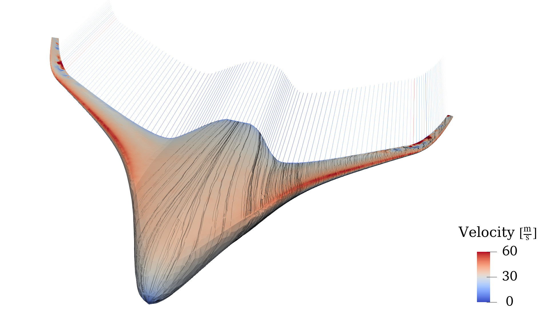
# Calculate surface velocity U on the body
Us = pnl.calcfield_U(body, body)
# NOTE: Since the boundary integral equation of the potential flow has a
# discontinuity at the boundary, we need to add the gradient of the
# doublet strength to get an accurate surface velocity
# Calculate surface velocity U_∇μ due to the gradient of the doublet strength
UDeltaGamma = pnl.calcfield_Ugradmu(body)
# UDeltaGamma = pnl.calcfield_Ugradmu(body; sharpTE=true, force_cellTE=false)
# Add both velocities together
pnl.addfields(body, "Ugradmu", "U")
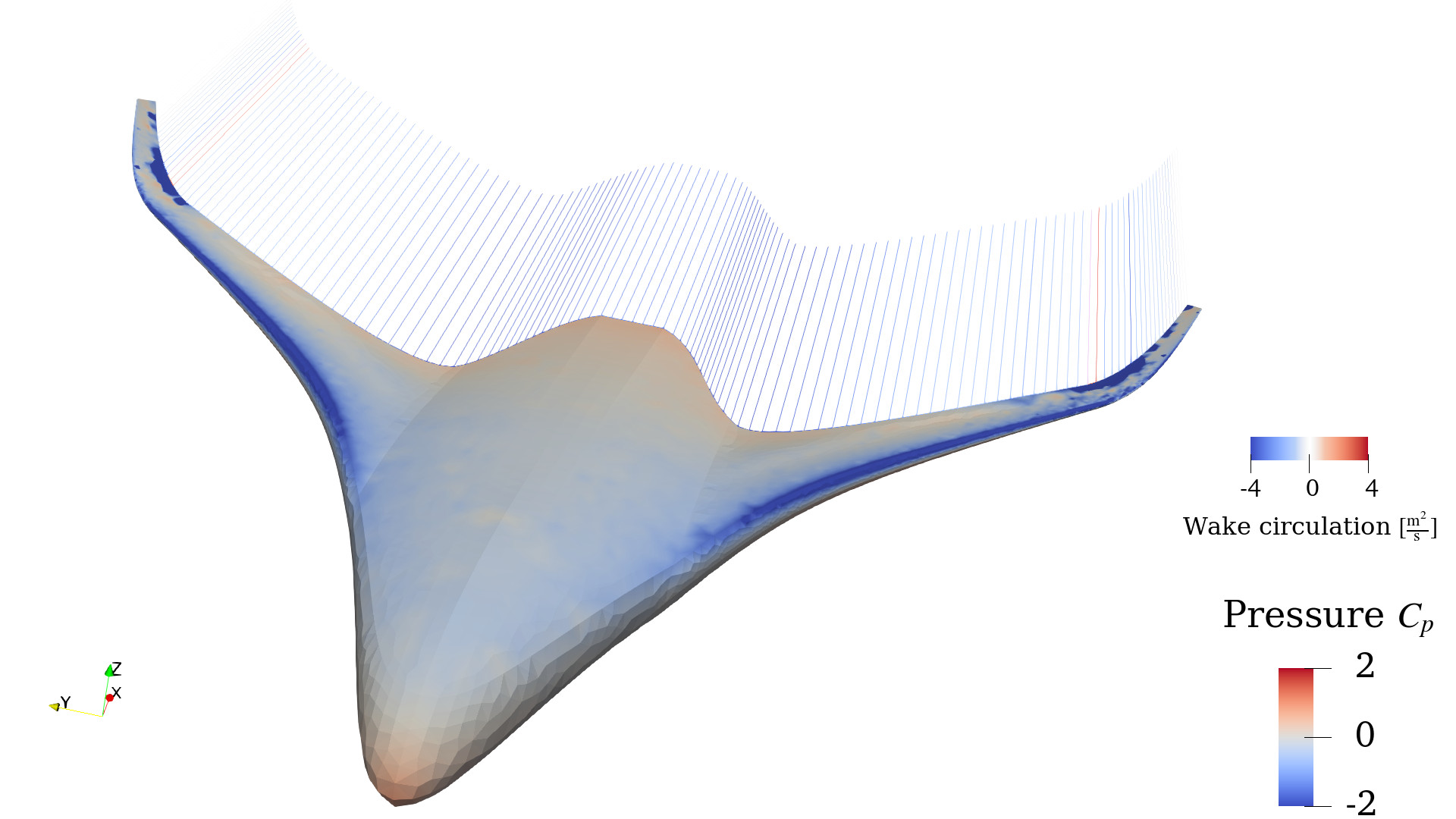
# Calculate pressure coefficient (based on U + U_∇μ)
@time Cps = pnl.calcfield_Cp(body, magVinf; clip = Cp -> max(clip_Cp, Cp))
# Calculate the force of each panel (based on Cp)
@time Fs = pnl.calcfield_F(body, magVinf, rho)
# Calculate total force of the vehicle decomposed as lift, drag, and sideslip
Dhat = Vinf/norm(Vinf) # Drag direction
Shat = [0, 1, 0] # Span direction
Lhat = cross(Dhat, Shat) # Lift direction
LDS = pnl.calcfield_LDS(body, Lhat, Dhat)
L = LDS[:, 1]
D = LDS[:, 2]
# Force coefficients
nondim = 0.5*rho*magVinf^2*Sref # Normalization factor
CL = sign(dot(L, Lhat)) * norm(L) / nondim
CD = sign(dot(D, Dhat)) * norm(D) / nondim
@show L
@show D
@show CL
@show CD
# ----------------- VISUALIZATION ------------------------------------------
# Save body as VTK
vtks = save_path*"/" # String with VTK output files
vtks *= pnl.save(body, run_name; path=save_path)
# Call Paraview
if paraview
run(`paraview --data=$(vtks)`)
endRun time: ~90 seconds on a Dell Precision 7760 laptop, no GPU (~10 seconds with GPU).
You can also automatically run this example with the following command:
import FLOWPanel as pnl

include(joinpath(pnl.examples_path, "blendedwingbody.jl"))- Check whether normals point into the body: Using the flag
debug=trueinpnl.save(body, run_name; path=save_path, debug=true)will output the control points of the body along with the associated normal vector of each panel. We recommend opening the body and control points in ParaView and visualizing the normals with the Glyph filter. Whenever the normals are pointing into the body, the user needs to flip the offset of the control points withCPoffset=-1e-14or any other negligibly small negative number. This won't flip the normals outwards, but it will flip the zero-potential domain from outwards back to inside the body (achieved by shifting the control points slightly into the body). If you pull up the solution in ParaView and realize that the surface velocity is much smaller than the freestream everywhere along the aircraft, that's an indication that the normals are point inwards and you need to setCPoffsetto be negative. - Check that the trailing edge was correctly identified:
pnl.save(body, run_name; path=save_path)automatically outputes the wake. We recommend opening the body and wake in ParaView and visually inspecting that the wake runs along the trailing edge line that you defined undertrailingedge. If not successful, increase the resolution oftrailingedgeand tighten the tolerance to something small likepnl.calc_shedding(grid, trailingedge; tolerance=0.0001*span). - Choose the right solver for the geometry: Use the least-squares solver with watertight bodies (
bodytype = pnl.RigidWakeBody{pnl.VortexRing, 2}), and the direct linear solver with open bodies (bodytype = pnl.RigidWakeBody{pnl.VortexRing}). The least-squares solver runs much faster in GPU (pnl.solve(body, Uinfs, Das, Dbs; GPUArray=CUDA.CuArray{Float32})), but it comes at the price of sacrificing accuracy (single precision numbers as opposed to double).